Книги по МРТ КТ на английском языке / MR Imaging in White Matter Diseases of the Brain and Spinal Cord - K Sartor Massimo Filippi Nicola De Stefano Vincent Dou

exam time increases linearly with TR. It is possible to perform more rapid imaging using short TR conventional spin-echo or gradient-echo sequences, but pure T2 contrast cannot be obtained. It should also be noted that the conventional spin-echo sequence is relatively inefficient in terms of data acquisition, because the majority of the time spent imaging is actually spent waiting for the decay of longitudinal magnetization.

The resolution to the quandary posed above was found in a pulse sequence that preserved the long time between excitations (TR) but made use of the “dead time” to acquire more data with which to construct an image. These data, taken together, constitute the “k-space” representation of the image.A basic understanding of this concept is easily gained and clearly illustrates the evolution from conventional to fast spin-echo imaging. Images obtained with fast spinecho (FSE, also called RARE and turbo spin-echo) techniques are now the most clinically essential. The ability to interpret and manipulate the contrast obtained with FSE is requisite to effective exploitation of the diagnostic capability.

In earlier chapters the development of gradientecho imaging was attributed in part to the advances in magnet and signal-processing technology that made it possible to obtain images without spin-echoes. In a similar manner, an ultra fast gradient-echo technique dubbed echo-planar imaging followed further technological developments. This again constituted a means of using most of the scan time to acquire data rather than wait for relaxation. It was also recognized that the spinand gradient-echo techniques could be combined in a variety of methods that offer opportunities to optimize the trade-offs between speed and quality.

4.2 k-Space

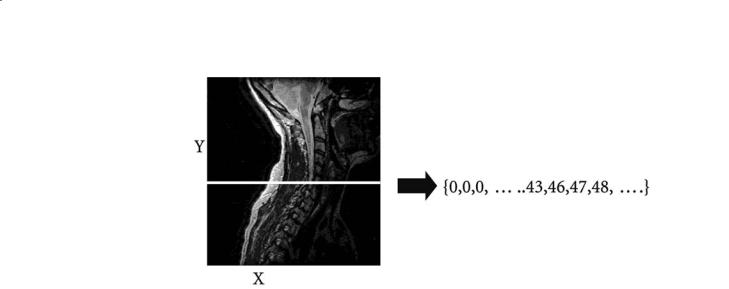
During MRI or any imaging examination, data is collected for future display.The display can be visualized as a collection of numbers corresponding to brightness (or gray scale) arranged in a (typically) square array or matrix. A possible approach in imaging is to acquire an individual point of data representing some feature of anatomy or function and to use that data value to fill in the intensity on the image matrix. Clearly,conventional X-ray imaging works in this way, even as all of the points are acquired simultaneously. If, for example, a problem with the X-ray film caused only half of the image locations to be obtained, the part of the image that was obtained would be perfect and indistinguishable from the corresponding part of a control image.Mathematically,it is said that there is a one-to-one correspondence between individual data points and spatial locations. It might be surprising to know that in magnetic resonance imaging, although it still true that the number of data points is equal to the number of image locations (picture elements, pixels), there is not a one-to-one correspondence. Rather, each data point that is acquired influences the entire image in some way. The image cannot be fully reconstructed (formed) without all of the data. Further, a mathematical process called the Fourier transform must be employed to translate the data into an image. Figure 4.1 is a diagram of this process in a “black box” sense.

Consider any MR image. If one wanted to send a perfect description of that image to a colleague, it would be possible to write down each pixel intensity on a gray scale from 0-256, agree in which order the numbers would be sent, and proceed to transfer the

a

Fig. 4.1. a The Fourier transform is used to process the data acquired in an MRI examination into an image. b Data acquired in an MRI imaging experiment is shown with the

Image reconstructed image. The acquired data is complex and the magnitude of that complex data is shown

numbers one at a time. The colleague could receive the numbers, reassemble the image into a matrix form (Fig. 4.2), and then display them as the gray scale equivalent. Clearly, an image is nothing more or less than a matrix of gray scale values (Fig. 4.2). In “image space”, one can select a particular location and note the intensity. The coordinates in image space are simply the standard spatial coordinates in the image plane.

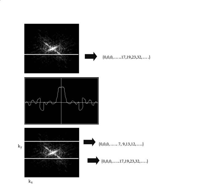
Similarly, the data collected in the MRI process is simply a list of numbers acquired over a length of time. During the examination, the voltages present in the RF coil are sampled and recorded by a computer. A voltage waveform of a particular frequency can be characterized by magnitude and phase and, typically, both parameters of the voltages are obtained using two radiofrequency channels. This is known as quadrature detection and results in data in socalled “complex” form. These data are assembled in what could be called the data matrix (Fig. 4.3). Each spin-echo can be recorded in this way as a collection of numbers including the approach to the echo as well as its decay. Successive spin-echoes with different strengths of phase encoding are recorded on their own line (Fig. 4.3c). Arranged in the data matrix (Fig. 4.3), the “locations” of individual data correspond to time, moving to the right with the progress of the spin-echo, and outward from the center with the integrated magnitude of the phase encoding gradient. Since the recording of the spin-echo is associated with the application of the “read” or fre- quency-encoding gradient, it is also correct to refer to the location with coordinates of integrated gradient magnitude. The center of the data matrix corresponds to zero gradient in both phase and frequency direction. It is the center, or peak, of the spin-echo acquired with zero phase encoding. Since stronger gradients contribute dephasing that in general low-

ers signal intensity, it is apparent that the center of the data matrix will have the largest intensity.

It may be seen at this point that the data matrix under discussion is no other than “k-space”, and that k-space is in some way an inverted form of image space. The coordinates of k-space can be thought of as times. The coordinates of image space are spatial in nature, but the gradients serve to establish a correspondence between frequency (or phase) and position. Thus, the coordinates of image space can be thought of as having units of frequency. It is useful to note that the k-space matrix is theoretically symmetric. Clearly, the ideal spin-echo is identical in buildup and decay, yielding, in conventional coordinates, the left-right symmetry of the matrix. Additionally, the magnitude of dephasing due to a phase encode gradient does not depend on the sign (direction) of the gradient. Thus, applying a “positive one unit” of phase encoding is theoretically identical to applying a “negative one unit”, and thus the matrix is symmetric top to bottom. This two-dimensional symmetry is exploited in some techniques that shorten acquisition time by acquiring only a part of the actual matrix and filling in missing data.

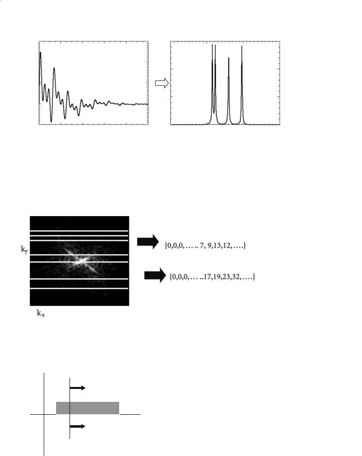
The Fourier transform, introduced above as a “black box”that changes the data matrix to the image, can be described in a number of ways. Fourier theory holds that any function in time (the signal, the spinecho) can be exactly described as the sum of sinusoidal functions. The individual sinusoids (of particular frequency) constitute the frequency components of the signal (Fig. 4.4) and the Fourier transform is simply a mathematical tool used to convert one to the other. Thus, in terms of signal processing, the Fourier transform serves to relate the time domain representation of a signal to its frequency domain equivalent. The theory can be extended to more than one dimension. In two-dimensional (2D) MRI, the 2D Fourier

transform serves to translate k-space to image space. The mechanics of doing so are handled quite efficiently and rapidly by modern computers.

A pulse sequence for MRI can be thought of as a scheme for “covering” k-space, that is, for acquiring data such that all point of k-space are known. The spin-warp sequence is perhaps easiest to understand as each horizontal line of k-space is completely filled by the acquisition of one spin-echo. Successive spinechoes with different phase encode values constitute the remaining lines and fill the matrix.When k-space is filled, the Fourier transform (albeit in two dimensions) of that matrix will directly yield the image (Fig. 4.5).

The k-coordinate, establishing the location in the k-space matrix, can be defined for constant gradients as:

where G is gradient strength as a function of time, γ is the gyromagnetic ratio, and t is the time of gradient application (Fig. 4.6). The read gradient controls kx and is turned on in conjunction with the collection of data.With the passage of time, Eq. (1) can be continuously evaluated as the k coordinate increases linearly. Similar “motion” in k space is associated with all gradient manipulations in the pulse sequence.

The k-space matrix can be filled line-by-line, as has been described above, or via less conventional means, including as a spiral outward from the center, simply by varying the application of gradients. As noted, application of a constant read gradient in the absence of a phase encode gradient is equivalent to moving to the right with time in the k-space matrix. Application of a constant phase encode gradient along with the read gradient would provide a diagonal motion. To move back to the left one would apply a negative read gradient. Curved paths would be real-

ized by more complex time-varying gradients. Some of these are desirable from the standpoint of accurate and physically realizable fast gradient switching. That is, one may choose a k-space trajectory based upon the physical limitations of the gradient amplifiers. The original echo-planar implementation (discussed below) is based upon applying to the gradient amplifiers the most basic waveform possible, a sinusoid. Curved trajectories may be less intuitive than the visualization of individual spin-echoes, but from the standpoint of the cumulative gradient effect they are relatively straightforward to interpret. The complicated k-space trajectories that are employed by modern pulse sequences, and indeed any k-space trajectories, can be created by controlling the gradients in this manner.

The contribution to the final image of specific data points may not be intuitively obvious, because

the form of the final image is not discernible from the appearance of the k-space matrix. However, the effect of a single data point on the entire image can be estimated and simulated. The nature of that effect is related to the position of the data point in the k- space matrix. The implications of this observation are profound and essential to the understanding of artifact as well as to the proper prescription of the imaging study. For example, an artifact featuring parallel stripes or a herringbone pattern may be seen on an image when a“pop”of static electricity is recorded during image data collection, and where only one or two points are abnormally high values. The orientation and number of the stripes are functions of the location of the bad point(s) in k-space (Fig. 4.7). This arises from the fact that each data point can be associated with a sinusoidal function that is part of the Fourier representation of the data, where the fre-

quency of the sinusoid (striping function) is higher for larger values of the k-coordinate.

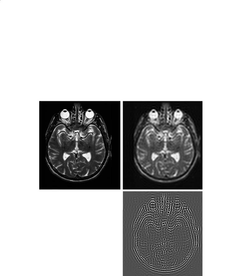
An accurate and simple generalization is that the central area of k-space contributes primarily to image contrast while the peripheral area of k-space contributes primarily to the definition of edges. This can be illustrated by the simulated reconstruction of an image using only a portion of the data, with the remaining data points set to zero. As can be seen in Fig. 4.8, a reconstruction using only 6% of the original data points results in a blurry yet interpretable image that would in some cases be diagnostic. Omitting the center data points yields an image that

shows only edges (Fig. 4.8c). These observations give rise to some techniques for rapid image acquisition (for example, so-called keyhole imaging where outer points are “reused” in subsequent images).

To summarize, the signal is acquired over time by sampling the voltage present in the radiofrequency coil. The frequency content of that signal reflects the encoding of the gradients, which establish a correspondence between frequency and spatial position. The Fourier transform is employed to convert the time-domain signal into the frequency domain information that is decoded into spatial position.

4.3

Spin-Echo Acquisition with Multiple Echoes

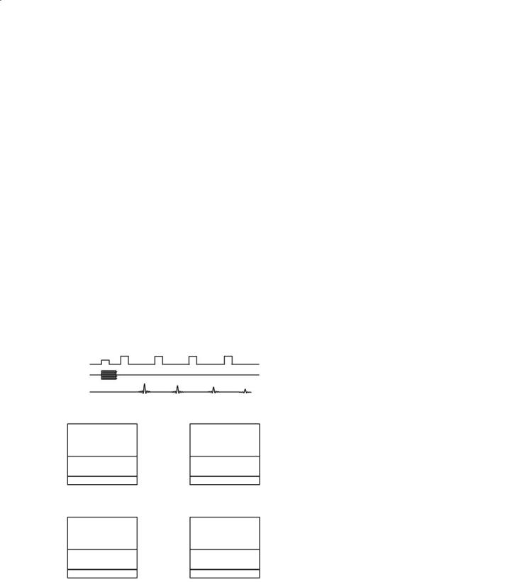
Recall that conventional spin-echo imaging can be used to obtain T2-weighted diagnostic images. A long repetition time (TR) must be used to allow for the recovery of longitudinal magnetization and to avoid T1 weighting. Proton density images are typically obtained in these studies because they come “free”, that is, without any time penalty. Specifically, the time spent collecting the data to acquire proton density images is completely contained within the time spent waiting for T1 decay. A slight extension of this technique gives the general “multiple spin-echo” acquisition, as discussed in Chap. 3 and diagrammed in Fig. 4.9. In this technique, the spin magnetizations are repeatedly refocused by successive inversion pulses. In the example four echoes are produced but more or fewer are possible. During each TR period, multiple lines of k-space data are acquired, one for each spin-echo that is formed. Each of these echoes is associated with the same phase-encode gradient, but they differ in echo time (TE). Thus, in each of the k-space matrices that correspond to specific echo times, the same line is filled in during the TR. The k-

RF

PE Gradient signal

a

Fig. 4.9a,b. In a multiple spin-echo sequence, one phase-en- code gradient application per TR is used (a). Four images are acquired when the PE gradient is incremented through full range, and the contrast in each image reflects the TE of the echo associated with that image. K-space maps are shown in (b) for the first TR period

space data are used to build up k-space matrices for each of the images as diagrammed in Fig. 4.9b. At the end of the acquisition there is enough information to reconstruct images for each of the TEs for which echoes were collected. A single completion of the acquisition sequence yields data for four images, and the time taken is the same as that required to collect data for the single longest image. This technique thus improves the efficiency of image data collection by yielding multiple images in the same time that would be required to obtain one. However, greater than two multiple spin-echo images, for example, series with TE values of 30, 60, 90, and 120 ms, have not typically been found to be clinically useful. The images that are most valuable are typically the long-TE (T2weighted) images and perhaps the very short TE (or proton-density weighted) images. Standard imaging protocols for many years included proton-density images whenever T2-weighted images were obtained, even though they might have been considered of limited utility. These images were considered “free” in that no time was added to the study to obtain them.

4.4

Fast Spin-Echo

Fast spin-echo imaging (originally called RARE, rapid acquisition with relaxation enhancement and also “turbo spin-echo”; Hennig and Friedburg 1986) was introduced to exploit the “available” time in the TR period and to apply this time to the acquisition of a single image rather than acquisition of many images. In principle, the idea is to take a multiple echo sequence as illustrated above, and instead of writing the four lines of k-space in four separate k-space matrices, to use them all in a single k-space matrix, which thus is filled four times faster. In order to accomplish this the phase encoding must vary between each of the echoes – otherwise the four lines of k-space will occupy the same points.

Clearly, the difficulty with this idea is that the four echoes yielding data have different values of TE. In fact, in FSE imaging the k-space matrix is filled with lines representing echoes that differ widely in TE. To understand how this is possible one must recall that only a small portion of k-space determines the contrast in the image, and that the contrast is the parameter that is expected to change most dramatically between echoes with different TE values. On the other hand, if the subject is stationary, one does not expect the edge information to change. Thus, in FSE imaging

there is not defined a single TE but rather an effective TE. The effective TE is the TE corresponding to the information obtained with low values of the phase encode (PE) gradient. Equivalently, the effective TE is the TE of the echoes where the dephasing due to the PE gradient is minimal, giving the higher intensity, central part of k-space. The decision regarding which echo to use for the contrast information is made automatically as part of the prescription of the pulse sequence when the effective TE is chosen.

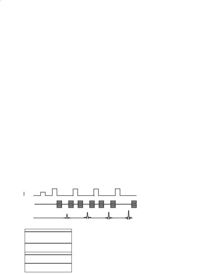
Consider FSE acquisition with four echoes. The rf excitation part of the pulse sequence is essentially identical to the four-echo multiple spin-echo sequence discussed above. The essential difference between the sequences is in the phase encoding gradient, applied before every echo. In each TR period, four lines of k-space are filled in the same image. An example is depicted in Fig. 4.10. Note in the example that the overall signal intensity increases over the TR period, that is, that the strongest echo is the last one. That may be counter-intuitive given that T2 decay (dephasing) progresses during TR, an effect that contributes to loss of signal over time. Pure T2 decay is indeed present and is irreversible but it is relatively slow on the time scale of interest. In contrast a largely reversible dephasing is contributed by field gradients, and it is this type of dephasing, specifically that of the phase encode gradient, that dominates the overall strength of successive spin-echoes in FSE imaging. Smaller values of PE gradient contribute less dephasing and thus result in stronger signals. In the example of Fig. 4.10 the value of the PE gradient decreases with successive echoes and thus the signal strength

RF

PE Gradient

signal

increases. In viewing this example, recall that negative gradient application can be used to decrease the overall integrated magnitude of any gradient. For completeness we note that T2* decay, the observed signal decay during the echo, includes magnet inhomogeneities that make up most of the observed dephasing of the individual spin-echo. This dephasing is to a large degree reversible and is in fact reversed when each spin-echo is formed.

Fast spin-echo can be employed with as many echoes as desired, as long as the signal is sufficient at the end of the sequence to allow collection of data. The number of echoes collected in each TR period is known as the echo train length (ETL) and represents the factor by which the total image acquisition time is divided. Equivalently, it is the factor by which the exam is speeded up. Repetition time (TR) is defined as in any pulse sequence and effective TE is defined as noted above. Echo spacing is defined as the time between successive echoes and any of these factors are determined by the other three. A useful relationship is:

a ETL

where Ta is the acquisition time, #PE is the number of phase encode steps and ETL is echo train length.

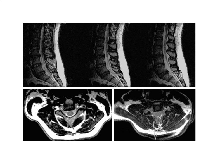
FSE imaging is now routine clinical practice and produces diagnostic quality T2-weighted images in brain and spine (Fig. 4.11). The choice of ETL and other timing parameters is made with consideration of local equipment and constraints. Typically the

Fig. 4.10. a In a fast spin-echo image, multiple phase encode gradient applications are used in each TR. One image is acquired after all phase-encode values are applied. b A k-space map for the first TR is shown. Here, the values of the phase-encode gradient are 120, –72, 56, –8. Ordering in this way makes the signal intensity of the echoes increase during TR, and makes the contrast of the resultant image reflect the later echo

quality of images obtained at any individual center will dictate the ETL, made, all else equal, as large as possible.

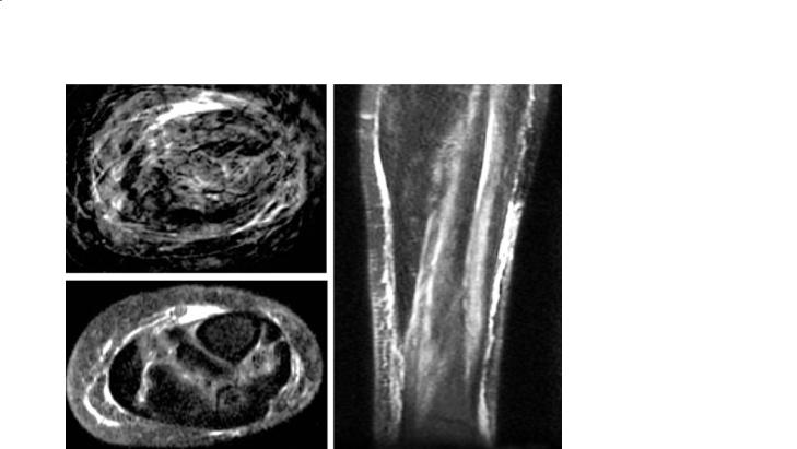
The ultimate extension of FSE is single-shot FSE (SSFSE), whereby the entirety of k-space is filled in following a single initial excitation (π/2) rf pulse. This pulse sequence actually has no TR value, since there is no repetition, but may require only tens of seconds. In current implementation the symmetry of k-space is exploited in SSFSE, with slightly more than half of the phase encode values sufficing to fill in the data matrix. The resulting images are of lower quality than generally expected for diagnostic images, but are highly useful for “go/no go” evaluation of certain lesions and particularly in patients whose ability to remain still is limited. As shown in Fig. 4.12, SSFSE was employed to produce a diagnostic image in an uncooperative patient where conventional SE and even FSE were simply too slow. Single-shot FSE in brain may not typically provide the quality needed by clinicians for routine evaluation, but continued improvements in scanner technology and signal processing should result in standard protocols featuring this technique.

4.5

Image Quality and Artifacts

A reasonable concern is the extent to which FSE images are equivalent to those acquired with conventional spin-echo techniques. Clearly, to make this comparison the images must be acquired with the FSE effective TE values equal to the conventional TE values. That being assumed, FSE images are in fact used like the conventional spin-echo images that they were designed to replace. However, some differences do arise from a number of physical factors. First, the signals that fill k-space do originate from spin-echoes with different values of TE, and the effects of pure T2 decay make those echoes different. In the case of FSE with the longest echoes assigned to the low phase encode values, the effect is minimized because the strongest echoes (low phase encoding) will be the least affected by T2 decay during the TR period. Thus, in FSE images with long effective TE, the image quality is highest because the high phase encode acquisitions, which are characterized by maximal dephasing and lowest signal strength, occur early in

the T2 process. These acquisitions provide the high spatial frequency edge information. In the alternate scenario, PD-weighted FSE, the higher phase encode acquisitions must be assigned to the later echoes. If signal strength is insufficient at this point in the sequence, the information from those echoes will be contaminated or dominated by noise, disrupting the reconstruction of edge information. The resulting images will be relatively blurred.

Another source of blurring common to all imaging modalities is described by the point-spread function, which relates the theoretical distribution of signal originating within a single pixel to adjacent pixels. In FSE, the point-spread function takes the form:

with FW representing the full width and half height of the function, this being a standard measure of linewidth such that a wider line corresponds to more “spread” of the information, hence more blurring. In this equation, ∆y is the pixel dimension, and the remaining parameters have been previously defined. A similar issue related to the point spread function is ringing artifact, manifest as repeating bands related to the discontinuous T2 weighting function. Again,

this artifact results from the fact that significant T2 decay can occur on the time scale of the phase encoding. Methods have been proposed and implemented to reduce these effects. The importance of the point spread function to the physician prescribing the MR scan is that the amount of blurring and ringing due to T2 decay can be controlled through the ETL and the Es.

Another concern in 2D FSE is magnetization transfer (MT). Consider that when multiple slices are prescribed, the data to reconstruct them is acquired in an interleaved fashion. Thus, the repetition time contains all of the echoes being acquired for one slice, and also the echoes for all slices in the study. For a given slice, the rf excitation for its adjacent slices can be considered“off-resonance”in the same sense as for the design of a magnetization transfer sequence. In conventional spin-echo, these effects are present but insignificant. In FSE, the rf pulses occur much more frequently. Here, the MT effects are measurable and tend to enhance the contrast achieved by T2 weighting. A related concern is the observation that many successive inversion pulses carry a heavy absorbed power load,and may be limited by United States Food and Drug Administration (FDA) or other government agency constraints. This limitation increases in severity with static magnetic field strength, and is of