Schluesseltech_39 (1)

focus on isotope-incoherence and leave the detailed discussion of spin-incoherence for other chapters.

Figure 4.11 shows a 2-D model crystal with atoms of two isotopes of the same element with two different scattering lengths bi sitting on fixed positions Ri in a crystal lattice. As stated above, the scattering amplitude is obtained from a Fourier transform:

i

When we calculate the scattering cross section, we have to take into account that the different isotopes are distributed randomly over all sites. Therefore, we have to average over the random distribution of the scattering length in the sample:

As isotopes of the same element are chemically undistinguishable, the distribution of the scattering lengths bi and bj on the different sites is completely uncorrelated. This implies that for i j, the expectation value of the product equals to the product of the expectation values. Only for i = j a correlation occurs, which gives an additional term describing the mean quadratic deviation from the average:

The scattering cross section is a sum of two terms. Only the first term contains the phase factors eiQ R, which result from the coherent superposition of the scattering from pairs of scatterers. This term takes into account interference effects and is therefore named coherent scattering. The scattering length averaged over the isotopeand nuclear spindistribution enters this term. This is in complete analogy to the “isotope insensitive” x- ray-diffraction. The second term in (4.16) does not contain any phase information and is proportional to the number N of atoms (and not to N2). This term is not due to the interference of scattering from different atoms and it has no direct counterpart in x-ray scattering. As we can see from (4.14) (line i = j), this term corresponds to the scattering from single atoms, which subsequently superimpose in an incoherent manner (adding intensities, not amplitudes!). This is the reason for the intensity being proportional to the number N of atoms. Therefore the second term is called incoherent scattering.

i C Interference

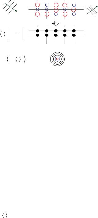
Fig. 4.11: Upper panel: Sketch of the scattering process from a 2-D lattice of N chemically identical atoms with two isotopes (small dotted circles and large hatched circles). The area of the circle represents the scattering cross section of the single isotope. Middle panel: The incident wave is scattered coherently only from the average structure. This gives rise to Bragg peaks in certain directions. Lower panel: Additionally, an isotropic background (incoherent scattering) is observed, which is proportional to the number N of atoms and to the mean quadratic deviation from the average scattering length.

The most prominent example for isotope incoherence is elementary nickel. The scattering lengths of the nickel isotopes are listed together with their natural abundance in Table 4.1 [2]. The differences in the scattering lengths for the various nickel isotopes are enormous. Some isotopes even have negative scattering lengths. This is due to resonant bound states, as compared to the usual potential scattering.

Tab. 4.1: The scattering lengths of the nickel isotopes and the resulting scattering length of natural 28Ni [2], see also fig. 4.9.

Neglecting the less abundant isotopes 61Ni and 64Ni, the average scattering length is calculated as:

which gives the total coherent cross section of:

The coherent scattering lengths of hydrogen (-3.74 fm) and deuterium (6.67 fm) are significantly different. This can be used for contrast variation by isotope substitution in all samples containing hydrogen, i. e. in biological samples or soft condensed matter samples, see the corresponding chapters.

A further important element, which shows strong nuclear incoherent scattering, is vanadium. Natural vanadium consists to 99,75 % of the isotope 51V with nuclear spin 7/2. By chance, the ratio between the scattering lengths b+ and b- of this isotope are approximately equal to the reciprocal ratio of the abundances. Therefore, the coherent scattering cross section is very small and the incoherent cross section dominates [2]:

For this reason, Bragg scattering of vanadium is difficult to observe above the large incoherent background. On the other hand, this fact can be turned into an advantage: By using vanadium metal, one can make sample containers which are practically invisible for (coherent) neutron scattering: They produce almost no reflections but rather a diffuse background (since incoherent scattering is isotropic) which usually doesn’t cause severe problems in diffraction experiments.

4.3 Diffraction geometry

For purely elastic scattering, the scattering function S(Q,@) reduces to the special case without energy transfer (E0 = E1 and I = E0 – E1 = 0) and equal length of the wave vectors of the incident and scattered beams (!k0! = !k1!). S(Q,@ = 0) and the scattering intensity then only depends on the scattering vector Q = k0 - k1. The coherent elastic neutron scattering ( neutron diffraction) yields information on the positions (distribution) of the atomic nuclei and the arrangement of the localised magnetic spins in crystalline solids, the pair correlation function of liquids and glasses, and the conformation of polymer chains.

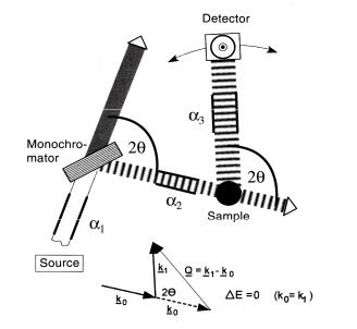
Figure 4.12 shows a sketch of a general diffraction experiment. More specifically, it is a typical setup of a constant wavelength, angular dispersive diffraction experiment. There are other methods to perform a diffraction experiment (e.g. time of flight- (TOF-), Laue-, energy-dispersive diffractometers etc.) but these are outside the scope of this introductory lecture.

For constant wavelength diffraction, the energy (wavelength) and direction (collimation) of the incident neutron beam needs to be adjusted. For that purpose, the diffractometer is equipped with a crystal monochromator to select a particular wavelength band (B ? EBJB) out of the “white” beam. Collimators are used to define the beam direction and divergence pretty much as is done in x-ray diffraction.

In the case of a crystalline sample, the diffraction geometry is most conveniently described by the concepts of the reciprocal lattice and the Ewald construction which are both well-known from x-ray-diffraction.

Fig. 4.12: Schematic representation of a constant wavelength diffractometer.

Reciprocal lattice

The characteristic feature of the crystalline state (see chapter 3) is its periodic order, which may be represented by a (translation) lattice. In the 3D case, three basis vectors a1, a2, a3 define a parallelepiped, called unit cell. Each lattice node of the crystal lattice can be addressed by a general lattice vector

which results from a linear combination of the basis vectors with coefficients u, v, and w (positive or negative integers, including 0).

The position of atom j in the unit cell is given by the vector

The coefficients xj, yj, and zj are called atomic coordinates (0Kxj<1; 0Kyj<1; 0Kzj<1). a2, a3 there is only

(4.25)

of the reciprocal lattice. h,k,l are the integer Miller indices and;1, ;2, ;3 are the basis vectors of the reciprocal lattice, satisfying the two conditions

The basis vectors of the reciprocal lattice can be calculated from those of the unit cell in real space

where > means the cross product, and Vc = a1 (a2>a3) is the volume of the unit cell. In solid state physics,

is used instead of ;

Here is a compilation of some properties of the reciprocal lattice:

L Each reciprocal lattice vector is perpendicular to two real space vectors: ;I < aj and ak (for i j, k)

LThe lengths of the reciprocal lattice vectors are M;iM = 1/Vc MajM MakM sinN(aj,ak).

LEach point hkl in the reciprocal lattice refers to a set of planes (hkl) in real space.

LThe direction of the reciprocal lattice vector ; is normal to the (hkl) planes and its length is reciprocal to the interplanar spacing dhkl: M;M = 1/dhkl.

LDuality principle: The reciprocal lattice of the reciprocal lattice is the direct lattice.

Performing a diffraction experiment on a single crystal actually means doing a Fourier transform of the 3D-periodic crystal (see chapter on symmetry in crystals) followed by forming the square of the resulting (complex) amplitude function. The Fourier transform of the (infinite) crystal lattice is essentially the reciprocal lattice derived above and yields directly the positions of the reflections in space (directions of the diffracted beams). The atomic arrangement within the unit cell determines the reflection intensities which may be envisaged as a weight attached to the nodes of the reciprocal lattice.

Doing a (single crystal) diffraction experiment therefore corresponds to measuring the positions and weights of the reciprocal lattice points. Their position yields information on the lattice parameters and the orientation of the crystal on the diffractometer while the weights (the reflection intensities) allow reconstructing the atomic positions within the unit cell.

Ewald construction

The concept of the reciprocal space also provides a handy tool to express geometrically the condition for Bragg scattering in the so-called Ewald construction. In this way the different diffraction methods can be discussed.

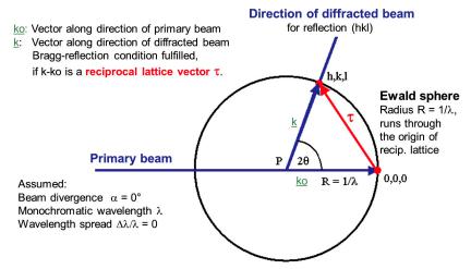
We consider the reciprocal lattice of a crystal and choose its origin 000. In Fig. 4.13 the wave vector k0 (defined in the crystallographers’ convention with Mk0M = 1/B) of the incident beam is marked with its end at 000 and its origin P. We now draw a sphere of radius Mk0M = 1/B around P passing through 000. Now, if any point hkl of the reciprocal lattice lies on the surface of this “Ewald sphere”, then the diffraction condition for the (hkl) set of lattice planes is fulfilled: The wave vector of the diffracted beam k (with its origin also at P) for the set of planes (hkl), is of the same length as k0 (MkM = Mk0M) and the resulting vector diagram satisfies k = k0 + ;. Introducing the scattering angle 2 (and

hence the Bragg angle hkl), we can deduce immediately from 2MkM sin = M;M the Bragg equation 2dhkl sin hkl = B.

Fig. 4.13: Ewald construction in reciprocal space, showing the diffraction condition for reflection (hkl).

In the case of single crystal diffraction a rotation of the crystal and therefore also of the corresponding reciprocal lattice (which is rigidly attached to the crystal) is often used to set the diffraction conditions for the measurement of intensities I(;).

If M;M > 2/B (then dhkl < B/2) the reflection hkl cannot be observed. This condition defines the so called limiting sphere, with center at 000 and radius 2/B: only the points of the reciprocal lattice inside the limiting sphere can be rotated into diffraction positions. Vice versa if B > 2dmax, where dmax is the largest interplanar spacing of the unit cell, then the diameter of the Ewald sphere is smaller than M;Mmin. Under these conditions no node of the reciprocal lattice can intercept the Ewald sphere. That is the reason why diffraction of visible light (wavelength O 5000 Å) can never be obtained from crystals. Bmin determines the amount of information available from a diffraction experiment. In ideal conditions Bmin should be short enough to measure all points of the reciprocal lattice with significant diffraction intensities.

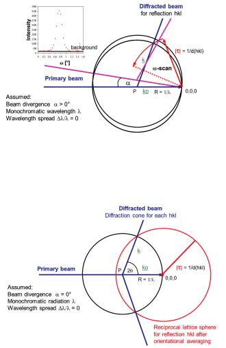
For a real crystal of limited perfection and size the infinitely sharp diffraction peaks (delta functions) evolve into broadened reflections. One reason can be the local variation of the orientation of the crystal lattice (mosaic spread) implying some angular splitting of the vector ;. A spread of interplanar spacings Ed/d, which may be caused by some inhomogeneities in the chemical composition of the sample, gives rise to a variation of its magnitude M;M. The ideal diffraction geometry on the other hand also needs to be modified: In a real experiment the primary beam has a non-vanishing divergence and wavelength spread. The detector aperture is also finite. A gain of intensity, which can be accomplished by increasing the angular divergence and wavelengths bandwidth, has to be paid for by some worsening of the resolution function

(see below) and hence by a limitation of the ability to separate different Bragg reflections.

All of these influences can be studied by the Ewald construction. The influence of a horizontal beam divergence on the experimental conditions for a measurement of Bragg-intensities of a single crystal is illustrated in Fig. 4.14 where strictly monochromatic radiation (only one wavelength B with EBJB = 0) is assumed. To collect the complete intensity contained in the spread out reflection, a so-called @-scan, where the crystal is rotated around the sample axis perpendicular to the diffraction plane, may be used. The summation over the whole reflection profile yields the so-called integral diffraction intensities.

Fig. 4.14: Ewald-construction: Influence of the horizontal beam divergence on the experimental conditions for the measurement of Bragg-intensities.

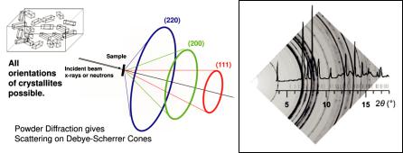
Finally, the geometry of powder diffraction experiments can also be discussed in terms of the Ewald-construction:

Fig. 4.15: Ewald construction for a powder diffraction experiment.

An ideal polycrystalline sample is characterised by a very large number of arbitrarily oriented small crystallites. Therefore, the reciprocal lattice point hkl is smeared out on a sphere and the 3D-information contained in vector ; is reduced to only 1D-information contained in M;M. In Figure 4.15 the corresponding sphere with radius M;M = 1/dhkl is drawn around the origin of the reciprocal lattice at 0,0,0. For each Bragg-reflection the circle of intersection of the “reciprocal lattice sphere” with the Ewald-sphere yields a diffraction cone. These cones are recorded on a point or position sensitive detector. And the resulting information is plotted as a intensity vs. diffraction angle (or Q) diagram. All reflections with equal interplanar spacing dhkl are perfectly superimposed and cannot be separated experimentally.

Fig. 4.16: Sketch of a powder diffraction experiment, diffraction cones are recorded on a 2Dor 1Ddetector (reproduced from [3]).

4.4 Diffraction intensities

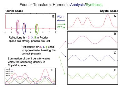
As stated in chapter 4.2, a scattering experiment is equivalent to performing a Fourier transform of the scattering object (eqn. 4.8) followed by taking the square of the resulting complex amplitude (eqn. 4.9). The latter step is very simply due to the fact, that our detectors can measure the magnitude (the absolute value) of a diffracted wave but are completely insensitive to its phase. This results in an intrinsic loss of information and poses the so-called “phase problem of crystallography”. There are methods to reconstruct the missing phase information from the measured magnitudes and from a-priori information about the scattering object (e.g. the so-called direct methods of structure determination), but these methods are again outside the scope of this lecture. The first step of a diffraction experiment - the Fourier transform - needs some further elaboration: In a diffraction (elastic, coherent scattering) experiment we can safely ignore time as a variable and concentrate only on the spatial Fourier transform of the scattering object (here: the crystal). For those who are not particularly familiar with the Fourier transform, figure 4.17 shows a very simple one-dimensional analogue. The transformation from A to E (labelled FT, ||) corresponds to the diffraction experiment: Fourier-transform (harmonic analysis) plus calculation of the absolute value. If we could also retrieve the phases , the inverse Fourier transform (labelled FT- 1, ) would lead directly to the structure of the scattering object A (harmonic synthesis).

Fig. 4.17: 1D illustration of the Fourier transform, A: scattering object: 1D-density function, assumed: periodic in 1D, B-D: decomposition of A into 3 harmonic (co-)sine waves, F: synthesis of A (red curve) via summation of B- D with the correct phases, E: “diffractogramm” of A: Fourier transform, only the magnitudes of waves in B to D are plotted, figures taken from[4].

Without the phase information, we need an approximate model of the crystal structure and a formula to calculate diffraction intensities from the model. In the kinematical approximation (see above) we use the so called structure factor formula for that purpose (see below). The model is then iteratively improved to give an optimum match between observed and calculated intensities. This is referred to as the structure refinement.

Structure factor and Bragg intensities

In the kinematical approximation, which assumes that the magnitude of the incident wave amplitude is the same at all points in the specimen (this implies a small sample size, weak scattering intensities, no multiple diffraction and negligible absorption), the diffracted intensity is proportional to the square of the amplitude of the scattered wave for each individual reflection; it can be regarded as a weight ascribed to the reciprocallattice nodes (see eqn. 4.25).

The structure factor F(;) is the Fourier transform of the scattering density within the unit cell. For a 3D-periodic scattering density function composed of discrete atoms (the crystal), the integral in (4.8) describing the Fourier transform in its most general form, simplifies to a sum over all atoms j in the unit cell The structure factor F(;) contains the complete structural information, including the atomic coordinates rj = xj a1 + yj a2 + zj a3 (see eqn. 4.24), site occupations and the thermal vibrations contained in Tj.