

Schluesseltech_39 (1)
.pdf5.24 |
H. Frielinghaus |
|
|
Fig. 5.14: The theoretical Debye function describes the polymer scattering of independent polymers without interaction. The two plots show the function on a linear and double logarithmic scale.
Fig. 5.15: Scattering of a h/d-PDMS polymer blend. The linear scale shows different compositions of hydrogenous polymer (from bottom to top: 0.05, 0.94, 0.27, 0.65) while the double logarithmic plot shows the 0.65 sample only [8].
S(Q) |
N(1 − 31 Q2Rg2) |
for small Q |
(5.49) |
|
N · 2/(Q2Rg2) |
for large Q |
(5.50) |
The line 5.49 describes the conventional Guinier scattering of the overall polymer (compare eq. 5.35). The second line 5.50 describes a power law. At these length scales the sub-chains of different lengths are self-similar and so they reveal a fractal behavior. The prefactor is connected to the magnitude Rg2/N which is the effective segment size. From this magnitude one can calculate back to the local rigidity which is responsible for the effective segments.
When we want to compare experiments with this theory the best examples are obtained from polymer blends (Fig. 5.15). One could come to the conclusion that diluted polymer solutions must provide the ideal conditions for such an experiment but practically the interactions of the solvent molecules with the monomers lead to a deviating behavior: The good solvent conditions lead to energetic violations of monomer-monomer contacts and so the polymer swells and displays a different fractal behavior. The high Q power law in good solvents comes close to Q−1.7. The Flory theory was the first attempt to describe this behavior while many refinements find small corrections. The theoretically most precise Flory exponent is ν = 0.588 which is the reciprocal value of the given exponent 1.7 above.
So polymer blends are often better examples for weakly interacting chains. This finding is supported by the low entropy of mixing which enforces small interactions. The discussed example of Fig. 5.15 [8] considers the isotopic mixture of hydrogenous and deuterated polydimethylsiloxane (PDMS). This practically leads to one of the lowest possible interactions even though they are not completely zero. The theoretical concept of the random phase approximation is able to deal with interactions and describes phase diagrams and the scattering in this way. At
Nanostructures investigated by SANS |
5.25 |
|
|
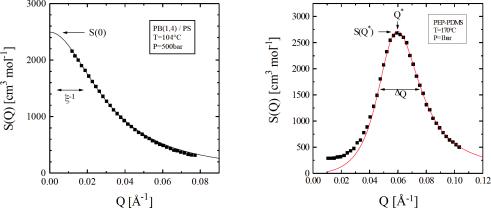
Fig. 5.16: Typical scattering of a homopolymer blend with interactions. The sample is a polybutadiene(1,4) / polystyrene blend at 104◦C and 500bar [9].
Fig. 5.17: Typical scattering of a diblock copolymer blend with interactions [10]. The poly-ethylene-propylene–poly- dymethylsiloxane is heated to 170◦C (1bar).
high temperatures the polymers usually mix well, and the scattering comes closer to the weakly interacting case. Closer to the demixing temperature at lower temperatures the scattering intensity increases dramatically. This indicates strong composition fluctuations. The system loses the tendency to form a homogenous mixture and so local enrichments of species A or B are possible. While the random phase approximation is a mean field concept which describes weak fluctuations there are other concepts for strong fluctuations close to the phase boundary: The 3-dimensional Ising model – known for ferromagnets – describes the strong fluctuations of the two component polymer system.
The example of an interacting homopolymer blend is shown in Fig. 5.16. The general aspects are kept from non-interacting polymers (compare Fig. 5.15). The scattering curve has a maximum at Q = 0, and is decaying to large Q where a power law of Q−2 for ideal chains is observed. The maximal intensity is connected to the reciprocal susceptibility which describes the tendency of spontaneous thermal fluctuations to decay. High intensities mean low susceptibilies and strong fluctuations – the vice versa arguments are valid. The width of this curve is connected to the correlation length ξ. At low interactions it is tightly connected to the single coil size, i.e. Rg. With strong fluctuations close to the phase boundary the correlation length tends to diverge, which measures the typical sizes of the thermally fluctuating enrichments.
A diblock copolymer is a linear chain with two different monomer species. The first part is pure A and the latter pure B. The typical scattering of a diblock copolymer blend is shown in Fig. 5.17. At small Q the ideal scattering increases with Q2 accordingly to the ‘correlation hole’. The chemistry of the molecule does not allow for enrichments of A or B on large length scales. A continuously growing volume would only allow for enrichments on the surface – this explains finally the exponent in the scattering law. The experimental finite intensities relate to imperfections of the molecules. The chain length ratio f is distributed, and finally allows for enrichments on large length scales.

5.26 H. Frielinghaus
The dominating fluctuations are found at a finite Q . This expresses that the coil allows for separations of A and B predominantly on the length scale of the overall coil. Close to the phase boundary and especially below (where the polymer undergoes a micro phase separation) the coils are stretched. The peak at finite Q also expresses that the fluctuations tend to form alternating enrichments. From a center it would look like a decaying order of A-B-A-B-... The
width of the peak is again connected to the |
correlation length |
ξ |
Q |
−1 |
which describes the |
||
|
|||||||
|
−2 |
|
|
||||
length of this decaying order. At high Q, again a Q |
|
law is observed describing the sub-chains |
|||||
being ideal chains. On these length scales homopolymer blends and diblock copolymers do not differ.
The whole understanding of phase boundaries and fluctuations is important for applications. Many daily life plastic products consist of polymer blends since the final product should have combined properties of two different polymers. Therefore, polymer granulates are mixed at high temperatures under shear in an extruder. The final shape is given by a metal form where the polymer also cools down. This process involves a certain temperature history which covers the one-phase and two-phase regions. Therefore, the final product consists of many domains with almost pure polymers. The domain size and shape are very important for the final product. So the process has to be tailored in the right way to yield the specified domain structure. This tailoring is supported by a detailed knowledge of the phase boundaries and fluctuation behavior. Advanced polymer products also combine homopolymers and diblock copolymers for an even more precise and reproducible domain size/shape tailoring [11, 12]. The diblock copolymer is mainly placed at the domain interfaces, and, therefore, influences the domain properties precisely.
5.3.4 The structure factor
In this section we develop the ideas about the structure factor – an additional factor for the scattering formula (eq. 5.32) – which describes the effect of interactions between the colloids or particles. We start from a rather simple interaction for colloids. It simply takes into account that the particles cannot intersect. This interaction is called excluded volume interaction. Then the general case will be discussed briefly and conceptually.
We start from the scattering length density for two spheres with different origins R1 and R2. In this case the formula reads:
ρ(Q) |
= |
|
ρ · Vsphere · exp(iQR1) + exp(iQR2) · K(Q, R) |
(5.51) |
|||
K(Q, R) |
= |
3 |
· |
|
sin(QR) − QR cos(QR) |
(5.52) |
|
(QR)3 |
|||||||
|
|
|
|
|
|||
The main difference arises from the phases of the two origins of the two colloids. Otherwise the result is known from eq. 5.31. For the macroscopic cross section we rearrange the amplitudes in the following way:
Nanostructures investigated by SANS |
5.27 |
|
|
|
(Q) = (Δρ)2 · |
|
· Vsphere · |
|
exp(iQR1) |
|
· |
|
|
|
|
1 + exp(iQ R) |
|
|
R · K2(Q, R) |
dΩ |
Vtot |
2 |
|||||||||||||
dΣ |
2Vsphere |
|
|
|
|
1 |
|
2 |
(5.53) |
||||||
|
|
|
|
|
|
|
|
|
|
|
|
|
|
|
|
There are factors for the contrast, the concentration, the single particle volume, one phase factor which results in 1, one factor for the relative phases, and the form factor. In comparison to eq. 5.32 all factors are known except for the factor about the relative phases. The brackets describe an ensemble average known from statistical physics. We have to consider all possible relative positions R. This is done in the following:
S(Q) = |
|
2 |
1 + exp(iQ R) 2 |
R = |
1 + cos(Q R) |
R |
|
|
|
1 |
|
|
|
|
|
|
|
|
|
|
|
|
|
= |
Vtot |
Vtot + 2πδ(Q) − 3 (2R)3K(Q, 2R) |
|
||||
|
1 |
|
|
4π |
|
|
|
(5.54)
(5.55)
The main result is found in line 5.55 which is obtained from the ensemble average. The prefactor arises from the normalization. The constant term arises from integrating over the whole volume. To be more precise the vector R has to omit a volume of a sphere with the radius 2R, because this is the minimum distance of the two centers. For the integral of the constant contribution we neglect this small difference. For the integral over the cosine function we have to do a trick which is called the Babinet principle: The really allowed volume is the sum of the full volume minus the sphere with the radius 2R. The cosine function integrated over the full volume is again a delta function, and the subtracted term is the Fourier transformation of a sphere, i.e. K(Q, 2R). We obtain the same result for the cosine-Fourier transformation and the complex Fourier transformation because the volume is centro-symmetric. The Babinet principle actually uses the inversion of the volume and states for squares of amplitudes, i.e. intensities, exactly the same result as for the original structure. For the structure factor we have to keep in mind: It arises from a single Fourier transformation and is not squared. The final result in brief is (neglecting the delta function again):
S(Q) |
= |
1 − φ2R · K(Q, 2R) |
(5.56) |
|
dΣ |
(Q) |
= |
(Δρ)2 · φsphere · Vsphere · S(Q) · K2(Q, R) |
(5.57) |
|
||||
dΩ |
||||
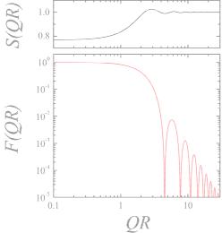
So we obtain the well known factors for the macroscopic cross section – now with a structure factor. The form and structure factor are compared in Fig. 5.18. The reduced intensity at small scattering vectors due to the structure factor appears for repulsive interactions and means that the possible fluctuations of the particles are reduced because they have less freedom. The first maximum indicates a preferred distance between the colloids. Such a maximum becomes more pronounced with higher concentrations. Note that for this example the maximum appears at a Q where the form factor already has a downturn. There are many examples in the literature where the form factor is still relatively close to 1 and then the structure factor is exposed very clearly.
5.28 |
H. Frielinghaus |
|
|
Fig. 5.18: The structure factor S(Q) on top of the form factor F (Q) = K2(Q). Note that the structure factor is smaller than 1 for small Q. This indicates a repulsive interaction. The first maximum of the structure factor expresses a certain tendency for preferred distances. Of course it only appears for rather strong concentrations.
So far we have derived the excluded volume structure factor for very dilute systems. The method of Ornstein-Zernicke allows for a simple refinement by describing higher order correlations on the basis of the simple pair correlation. Then – in the simplest way – one would obtain the following expression:
S2(Q) = 1 + φ2R · K(Q, 2R) −1 |
(5.58) |
A more rigorous treatment of the Ornstein-Zernicke formalism results in the Perkus-Yevick structure factor [13] which is the best known approximation for hard spheres. On the basis of this structure factor as the dominating term small corrections for additional interactions can be included [14]. For colloidal systems this is the strategy of choice.
Nonetheless, we would like to understand the structure factor more generally. From equation 5.54 we have seen that the phases of two centers have to be considered. The ensemble average finally took the distribution of possible distance vectors R into account. So we can understand the structure factor on the basis of a pair correlation function for the centers of the particles.
S(Q) = 1 + φ |
d3r |
g(r) − 1 exp(iQr) |
(5.59) |
V |
|
|
|
The function g(r) is the pair correlation function and describes the probabilities for certain distance vectors r, and the exponential function accounts for the phases. Again, for centrosymmetric g(r) there is no difference between a cosine and a complex Fourier transformation. The subtraction of the constant 1 accounts for delta peak contributions which we also obtained
Nanostructures investigated by SANS |
5.29 |
|
|
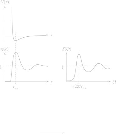
Fig. 5.19: The relation between the interaction potential V (r), the pair correlation function g(r) in real space, and the structure factor S(Q).
in line 5.55. The added term 1 we also obtained in the beginning (line 5.54). It arises from the self correlation of the particle with itself. For the pair distribution function we now can write:
g(r2 − r1) = |
P (r1, r2) |
, |
and φ = P (r1) |
(5.60) |
P (r1) · P (r2) |
and can be obtained theoretically with methods from statistical physics. It describes the probability for finding two particles at a distance r2 −r1. A rather elementary example is discussed in Fig. 5.19 starting from an interaction potential V (r). It has a repulsive short range interaction, a weak minimum at a distance rnn, and a quickly decaying tail to long distances. The distance rnn indicates the preferred distance of nearest neighbors. The pair correlation function then shows an inhibited range at short distances – similar to an excluded volume interaction. The following peak at rnn indicates a preferred nearest neighbor distance. The following oscillations for larger distances indicate more remote preferred places. The limit of g(r) at large distances is 1 indicating the average concentration of particles. For the structure factor we obtain a rather strong suppression at small Q. This means that the repulsive interactions lead effectively to a more homogenous distribution of particles. The peak of the structure factor at Q = 2π/rnn indicates the preferred distance of the nearest neighbors. Strong oscillations at higher Q indicate a narrow distribution of the actual neighbor distances. The limit at high Q is again 1, and arises from the self correlation of identical particles. This example describes a liquid-like behavior which has historically been developed for liquids. In soft matter research this concept applies for many systems ranging from colloids, over micelles to star-polymers. While the liquid-like structure describes a near order, a perfect crystal would lead to a different behavior: The correlation function g(r) would contain a lattice of separated delta peaks. The structure factor would
5.30 |
H. Frielinghaus |
|
|
describe the reciprocal lattice with the well known Bragg peaks. In soft matter research there exist many examples with liquid crystalline order. Very often they display a finite size of crystalline domains – so there is a grain structure – and the real state takes an intermediate stage between the perfect crystalline and liquid-like order.
5.3.5 Microemulsions
In this section we will follow a very successful way of deriving the scattering formula for bicontinuous microemulsions (see Fig. 5.20). Bicontinuous microemulsions consist of equal amounts of oil and water. A certain amount of surfactant is needed to solubilize all components, and a one phase system is obtained. The domain structure of the oil is a continuous sponge structure which hosts the water and vice versa. The surfactant forms a film at the surface between the oil and water domains.
The starting point is a thermodynamic model for such kind of system. The Landau approach takes mesoscopic sub-volumes and assumes that the internal degrees of freedom are integrated out, and there is a small number of order parameters describing the state of the sub-volume very accurately. For microemulsions we stay with a single (scalar) order parameter φ(r) which takes the values −1 for oil, 0 for surfactant, and +1 for water. Now the order parameter can still be treated like a continuous function since the physical effects take place on larger length scales than the sub-volume size. The (free) energy of the overall volume is now expressed as a function of the order parameter. One still cannot be perfectly accurat, so an expansion with respect to the order parameter is used. The expansion for microemulsions looks like:
F0 φ(r) = d3r c( 2φ)2 + g0( φ)2 + ω2φ2 (5.61)
This expansion does not only contain the order parameter itself, but there are derivatives included. These appear since this expression of the free energy is a functional expansion. Certain orders (especially the odd orders) of the order parameter and its derivatives have been ruled out due to the symmetry of the system. One important symmetry is the restriction to equal amounts of oil and water. Another facilitating property is that the functional form only considers local contributions in the functional form. For this free energy expression one can apply statistical physics methods and derive a scattering function (done in Appendix C). In comparison with the real space correlation function one can identify two important parameters: the correlation length ξ and the wavevector of the domain spacing k = 2π/d. The obtained scattering function looks like:
dΩ(Q) TS |
= (Δρoil−water)2 |
(k2 + ξ−2)2 |
|
2(k2 |
|
ξ−2)Q2 |
+ Q4 |
(5.62) |
||
dΣ |
|
|
8πφoil |
φwater/ξ |
|
|
||||
|
|
|
− |
|
|
− |
|
|
|
|
|
|
|
|
|
|
|
|
|
|
|
This function is also known as the Teubner-Strey formula [15]. While the applied concept approaches the reality as a long wavelength description, there are details missing. The described domains have rather plain walls while in reality the domain walls also fluctuate quite heavily. An empirical approach for the scattering function for the full Q-range is the following:
Nanostructures investigated by SANS |
5.31 |
|
|
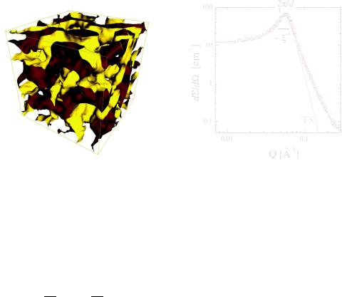
Fig. 5.20: A real space picture of the bicontinuous microemulsion according to computer simulations [16]. Actually the surfactant film is shown with the surface color being red for oil facing surface and yellow for water facing surface.
Fig. 5.21: The macroscopic cross section of a bicontinuous microemulsion. The peak indicates an alternating domain structure with the spacing d. The peak width is connected to the correlation length ξ. The grey line is the simple Teubner-Strey fitting while the red line corresponds to eq. 5.63.
dΣ(Q) = dΣ dΩ dΩ
TS |
|
|
1.5 Q4Rg4 |
||||
(Q) |
+ |
G erf12 |
(1.06 |
· QRg/√ |
6) |
||
|
|
|
|
· |
|
|
|
|
|
|
|
|
|
|
|
· exp −σ2Q2 |
(5.63) |
The error function erf(x) in the overall context describes a peak with a Porod behavior at large Q. This additional Porod term accounts for the larger surface of the fluctuating membranes. The final Gaussian factor describes a roughness of the surfactant film and often is not that clearly observed due to the high incoherent background. An example fit of this function to scattering data is discussed in Fig. 5.21. The pure Teubner-Strey function clearly shows a downturn at higher Q and the real Porod scattering is not well described. Only the additional Porod scattering allows for a realistic estimation of the averge surface of the domain structure.
From the structural parameters k = 2π/d and ξ one can make connections to the microscopic parameters of the microemulsion. The Gaussian random field theory describes the thermodynamics of a microemulsion by using a wave field that places the surfactant film at the zero surfaces of the field. The theory makes a connection of the structural parameters to the bending rigidity:
κ |
|
5√ |
|
|
|
= |
3 |
· kξ |
(5.64) |
||
kBT |
64 |
||||
The bending rigidity κ is an elastic modulus of the surfactant membrane. The overall underlying concept only relies on the elastic properties of the membrane to describe the thermodynamics
5.32 |
H. Frielinghaus |
|
|
Fig. 5.22: The sample position of the SAXS instrument ID2 at the ESRF, Grenoble, France. The photons propagate from the right to the left. The collimation guides on the left and the detector tank window on top of the cone on the left give an impression about the small beam size (being typically 1×1mm2).
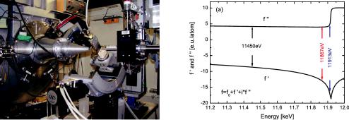
Fig. 5.23: The complex dispersion curve for gold (Au) at the L3 edge [17]. The overall effective electron number f = f0 + f + if replaces the conventional electron number Z = f0 in equation 5.65. On the x-axis the energies of the x-rays is shown, with indications for the experimentally selected three energies (black, red, blue). In this way, equal steps for the contrast variation are achieved.
of bicontinuous microemulsions. For symmetric amphiphilic polymers it was found that the bending rigidity increases [7]. The reason is that the mushroom conformation (obtained by the contrast variation measurements from chapter 5.3.2) exerts a pressure on the membrane. This makes the membrane stiffer which in turn allows to form larger domains with a better surface to volume ratio. So the much lower demand for surfactant is explained on the basis of small angle neutron scattering experiments.
5.4Small angle x-ray scattering
While a detailed comparison between SANS and SAXS is given below, the most important properties of the small angle x-ray scattering technique shall be discussed here. The x-ray sources can be x-ray tubes (invented by Rontgen,¨ keyword Bremsstrahlung) and modern synchrotrons. The latter ones guide fast electrons on undulators which act as laser-like sources for x-rays with fixed wavelength, high brilliance and low divergence. This simply means that the collimation of the beam often yields narrow beams, and the irradiated sample areas are considerably smaller (often smaller than ca. 1×1mm2). A view on the sample position is given in Fig. 5.22 (compare Fig. 5.3). One directly has the impression that all windows are tiny and adjustments must be made more carefully.
The conceptual understanding of the scattering theory still holds for SAXS. For the simplest understanding of the contrast conditions in a SAXS experiment, it is sufficient to count the electron numbers for each atom. The resulting scattering length density reads then (compare eq. 5.16):
Nanostructures investigated by SANS |
|
5.33 |
|
|
|
|
|
|
re |
|
|
|
|
|
|
ρmol = |
|
Zj |
(5.65) |
Vmol |
|||
|
|
j{mol} |
|
The classical electron radius is re = e2/(4π 0mec2) = 2.82fm. The electron number of each atom j is Zj. This means that chemically different substances have a contrast, but for similar substances (often for organic materials) it can be rather weak. Heavier atoms against light materials are much easier to detect. Finally, the density of similar materials is also important. Especially for organic materials (soft matter research), the high intensity of the source still allows for collecting scattering data. Many experiments base on these simple modifications with respect to SANS, and so the fundamental understanding of SAXS experiments does not need any further explanation.
For completeness, we briefly discuss the scattering length density for light scattering. Here the polarizability plays an important role. Without going into details, the final contrast is expressed by the refractive index increment dn/dc:
ρmol = |
2πn |
· |
dn |
(5.66) |
|
|
|
|
|||
λ2 |
dcmol |
||||
The refractive index increment dn/dc finally has to be determined separately experimentally when the absolute intensity is of interest. The concentration cmol is given in units volume per volume (for the specific substance in the solvent). The wavelength of the used light is λ.
5.4.1 Contrast variation using anomalous small angle x-ray scattering
While for contrast variation SANS experiments the simple exchange of hydrogen 1H by deuterium 2H ≡ D allowed for changing the contrast without modifying the chemical behavior, in contrast variation SAXS experiments the applied trick is considerably different: The chemistry is mainly dominated by the electron or proton number Z and isotope exchange would not make any difference. The electron shells on the other hand have resonances with considerable dispersion curves. An example is shown in Fig. 5.23 with the real part f (called dispersion) and the imaginary part f (called absorption). The overall effective electron number f = f0 + f + if replaces the conventional electron number Z = f0 in equation 5.65. Below the resonance energy the considered L3 shell appears only softer and effectively less electrons appear for f. Above the resonance energy single electrons can be scattered out from the host atom (Compton effect). This is directly seen in the sudden change of the absorption. Furthermore, the actual dependence of the dispersion is influenced by backscattering of the free electrons to the host atom (not shown in Fig. 5.65). This effect finally is the reason that the complex dispersion curve can only theoretically be well approximated below the resonance (or really far above). For this approximation it is sufficient to consider isolated host atoms.
For best experimental results the f-values have to be equally distributed. Thus, the energies are selected narrower close to the resonance (see Fig. 5.65). The investigated sample consisted of core-shell gold-silver nanoparticles in soda-lime silicate glass (details in reference [17]). By the contrast variation measurement one wanted to see the whole particles in the glass matrix, but also the core-shell structure of the individual particles. Especially, the latter one would