

Schluesseltech_39 (1)
.pdf5.44 |
H. Frielinghaus |
|
|
E5.2 The Pin-Hole Camera
The condition for the pinhole geometry is that the solid angle of the pin-hole observed from the position of the detector is equal or smaller than the solid angle of the object, here: the entrance aperture. Assume a symmetric SANS instrument with equal distances between the entrance aperture and the pin-hole (and sample), and between the pin-hole and the detector.
What is the ratio of the entrance aperture and the pin-hole dimensions?
|
a) |
2 |
|
b) |
3 |
|
c) |
4 |
What is the ratio of the areas? |
|
|
|
|||||
|
a) |
2 |
|
b) |
3 |
|
c) |
4 |
Assume that the eye operated as a pin-hole camera. The sizes may be for the aperture 1mm, for the retina distance 2cm, and for the object 1km.
What would be the minimal object size that could be resolved at this distance?
|
a) |
10m |
|
b) |
50m |
|
c) |
200m |
Why do we see better? |
|
|
|
|
|
|
||
|
a) |
aperture smaller |
|
b) |
eye contains lens |
|
c) |
we do not see better |
E5.3 Understanding of the Manuscript
The correlation function for a microemulsion is given in real space by eq. 5.93 and in reciprocal space by eq. 5.62. They describe an oscillating structure with the wavevector k and a correlation length ξ. A simpler correlation function is already obtained by equations 5.24 (real space) and 5.79 (reciprocal space, exact formula). Here, only a decaying correlation function is assumed in real space.
Which value does the k-vector of the first case take to obtain identical results?a) k = ∞ b) k = ξ−1 c) k = 0
In the structure factor of spherical colloids, the double radius 2R occurs for the simplest approximation in the effective concentration and the Q-dependent term K(Q, 2R) (see eq. 5.56).
Why does the double radius occur in this description?
a) Here, only two colloids are considered. For three colloids 3R would appear.
b) The closest distance of two colloids is 2R.
c) The square of the amplitude arising in the intensity causes effectively a factor 2.
The Porod behaviour (see eq. 5.34) and the high-Q limit of a polymer (see eq. 5.50) are simple power laws Qα with α being −4 and −2 in the first and second case.
What do these power laws indicate?
a) The exponent indicates how sharp the effective particle is defined at its surface.
b) The dimensionality (3 for sphere, 1 for polymer) plus 1 directly determines α.
c) Self-similarity. The structure looks on different length scales identical.
Nanostructures investigated by SANS |
5.45 |
|
|
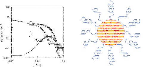
E5.4 Contrast Variation Experiment on Micelles
The three symbols , ◦, and indicate the characteristic small angle scattering of spherical polymer micelles under different important contrast conditions. There are three conditions called: shell contrast, core contrast and zero average contrast. The shell contrast highlights the shell of the micelle (being hydrogenated) while the rest is deuterated. The core contrast highlights the core of the micelle (being hydrogenated) while the rest is deuterated. For the zero average contrast the average contrast of the deuterated core and the hydrogenated shell matches with the solvent.
Which condition can be connected to which symbol (or curve)?
a) -shell ◦-core -zero b) ◦-shell -core -zero c) -shell -core ◦-zero Why?
E5.5 Spherical Form Factor
In microemulsions the topology of spherical droplets is quite frequent. We would like to assume a deuterated oil droplet of radius R surrounded by the protonated surfactant film and normal water (H2O). For simplicity, the oil is assumed to be homogenous with a scattering length density ρ, and the surrounding materials are assumed to have an average zero scattering length density (which is nearly true). So the amplitude ρ(Q) is calculated by the Fourier transform of a homogenous sphere. The macroscopic scattering cross section is normalized to the overall volume.
Calculate the three dimensional Fourier transformation of a solid sphere. Use spherical coordinates, and integrate in the order φ, ϑ, r. What is the simplicity of the integral over φ? How can the integral over ϑ be simplified (what is the variable X)? What does the kernel of the integral mean before the integration over r is performed? How would the integral be generalized for a scattering length density profile ρ(r) with spherical symmetry? What is the meaning of the term sin(Qr)/(Qr)?
5.46 |
H. Frielinghaus |
|
|
The formulas 5.28 to 5.33 already show the solution of the problem. Nonetheless, the student should be motivated to rationalize each step of the derivation. The highly motivated student might also derive the sphere scattering from eq. 5.22.
I thank my family and all my colleagues for supporting this  .
.
6Macromolecules (structure)
J. Stellbrink
Jülich Centre for Neutron Science 1
Forschungszentrum Jülich GmbH
Contents
6.1 |
Introduction....................................................................................... |
2 |
|
6.2 |
Polymers in dilute solution............................................................... |
2 |
|
|
6.2.1 |
Linear polymers......................................................................................... |
2 |
|
6.2.2 |
Branched polymers.................................................................................... |
5 |
|
6.2.3 In-situ experiments during polymerisation................................................ |
7 |
|
6.3 |
Block copolymer Micelles................................................................. |
9 |
|
|
6.3.1 |
Form factor ................................................................................................ |
9 |
|
6.3.2 |
Micellar exchange dynamics ................................................................... |
10 |
|
6.3.3 |
Structure factor ........................................................................................ |
11 |
6.4 |
Soft Colloids..................................................................................... |
12 |
|
Appendices |
................................................................................................. |
14 |
|
References .................................................................................................. |
|
15 |
|
Exercises..................................................................................................... |
|
16 |
|
________________________
Lecture Notes of the JCNS Laboratory Course Neutron Scattering (Forschungszentrum Jülich, 2011, all rights reserved)
6.2 |
J. Stellbrink |
6.1 Introduction
Macromolecules are an integral part of Soft and Living Matter. In Living Matter, macromolecule-based functional systems are built from molecular units consisting of only a few different building blocks: amino acids are assembled into proteins, which in turn function individually, or cooperatively in nanoand micro-machines. The secret of success is the intrinsic hierarchical structuring over a large range of length scales. In Soft Matter, synthetic macromolecules are of much simpler structure. Nevertheless, there is a vast variety of material properties that can be realized with synthetic macromolecules. Theoretical concepts have been developed, and are essential for the rational design of soft materials, that are of paramount importance in a multitude of technical applications.
Synthetic polymers have crucially changed daily life since its development in the 1930ies. Modern polymers can be divided into two major classes (i) commodity polymers for daily life use which are produced in millions of tons per year and (ii) specialty polymers for high-performance applications which are niche products but highly profitable [1]. Typical commodity polymers are polyolefines like polyethylene (PE) or polypropylene (PP) used for packaging, films etc. Examples for specialty polymers are polydimethylsiloxane (PDMS) derivatives used in dental implants.
Currently, both classes of polymers in use are based on petrochemical feedstock, thus considered not “carbon-neutral” and “environment-friendly”. Due to changing global conditions and growing concerns about the mounting disposal problems, research on sustainable commodity polymers has been intensified during the last decade, both on the level of fundamental research and applied science [2]. To find the required balance between material properties and bioavailability/-degradability is the key for establishing sustainable polymers on a large scale industrial level and therefore a major challenge of future polymer science.
The development of new biomimetic specialty polymers is another major challenge. Biopolymers, like spider silk, are high-performance materials with material properties superior to any synthetic polymer. To transfer these properties to artificial biomimetic polymers, one has to fully understand, on the molecular level, the structure-property- relationships and enzymatic synthesis processes in living organisms.
In this lecture some recent applications of neutron scattering methods to characterize quantitatively on a microscopic length scale structure and interactions of synthetic macromolecules and its hierarchical structuring are given. A more comprehensive overview is found e.g. in [3].
6.2 Polymers in dilute solution
6.2.1 Linear polymers
A linear polymer is a sequence of molecular repetition units, the monomers, continuously linked by covalent bonds. The degree of polymerisation, Dp, i.e. the number of monomers constituting the polymer, the (weight average) molecular weight, Mw=Dp Mm, with Mm the molecular weight of the monomer, and the radius of gyration, Rg ~ Mw , are the most important structural parameters of a polymer. On a coarse
grained level, structural details arising from the explicit chemical composition of the
Macromolecules (structure) |
6.3 |
polymer like bond lengths and angles can be neglected and what remains is the so called scaling relation given above that links molecular weight to size and which is generally valid for all polymers [4]. The numerical value of the scaling exponent depends on the strength of interactions. In the so called -state, when monomer-monomer interactions are as strong as monomer solvent interactions, the polymer structure can be described by a random walk, therefore Gaussian chain statistics are valid and =1/2, see Chapter 5.3.3. When monomer solvent interactions are stronger than monomer-monomer interactions, so called excluded volume forces are effective, the polymer chain is “swollen” and =3/5.
Here one has to emphasize that synthetic polymers, unlike biopolymers, always have an intrinsic polydispersity, i.e. there is a distribution of molecular weights. The polydispersity is given usually in terms of Mw/Mn, with Mn the number average molecular weight. Its precise number depends on the polymerisation reaction by which the polymer was synthesized. For a (theoretical) monodisperse polymer Mw/Mn=1 holds, the most monodisperse synthetic polymers with Mw/Mn=1.02 can be synthesized by “living” anionic polymerisation, classical polycondensation yields Mw/Mn =2, radical polymerisation can even result in extremely broad distributions, Mw/Mn >10.
Although in technical applications polymers are mostly used as bulk materials, polymer characterisation is usually performed in (dilute) solution. Historically, light scattering was the method of choice to characterise synthetic polymers [5], but nowadays size exclusion chromatography (SEC), also called gel permeation chromatography (GPC), is the standard technique to characterize routinely polymers [6].
Neutron scattering, due do its limited accessibility and high experimental costs, usually is found in basic academic research, but here it played a crucial role in confirming fundamental theoretical concepts of polymers [3].
As explained in detail in Chapter 5.3.4 the measured intensity I(Q)=P(Q) S(Q) is in first approximation a product of particle form factor P(Q) given by the intramolecular structure, i.e. the particle shape, and structure factor S(Q) given by the intermolecular structure arising due to particle-particle interactions. To characterize properly the intramolecular form factor P(Q) one has therefore to investigate a concentration series in the dilute regime and extrapolate finally to infinite dilution. The form factor of a Gaussian chain (Debeye function) has been derived in Chapter 5.3.3.
Particle-particle interactions as seen in S(Q) are weak in the dilute regime, but still effective, so that one can apply the virial expansion.
0 / I(Q 0) 1/Vw" 2A20 " |
(6.1) |
Here 05 is the polymer volume fraction and Vw Mw  d is the molecular volume and d
the polymer density in [g/cm3]. The value of the second virial coefficient A2 directly reflects particle-particle interactions, i.e. a positive A2 is found for repulsive interactions (good solvent), a negative one for attractive interactions (marginal/bad solvent) and finally A2=0 characterizes no interactions ( -solvent). Without any data fitting this distinction can easily be made by plotting the intensity data I(Q) of a concentration series normalized to the corresponding volume fractions I(Q)/ 0 (Since scattering arises due to an exchange of a volume element of solvent by a volume element of polymer with different scattering contrast, the natural concentration unit for any scattering

6.4 |
J. Stellbrink |
experiment should be volume fraction 0). This is schematically shown in Figure 6.1. If no particle-particle interactions are present all data for all Q-vectors exactly fall on top of each other.
-1 I[cm ]
-1 I[cm ]
-1 I[cm ]
Absolute intensity I(Q) [cm-1]
103
102 
1.8%
0.9%
101 |
10-2 |
10-1 |
Q [Å-1] |
|
|
100 |
4.3% |
|
2.6% |
|
|
10-1 |
|
|
103
102 |
|
|
101 |
|
|
100 |
4.3% |
|
|
2.6% |
|
|
1.8% |
|
10-1 |
0.9% |
10-1 |
|
10-2 |
|
|
Q [Å-1 |
] |
103
102 |
|
|
101 |
|
|
100 |
|
|
|
4.3% |
|
10-1 |
2.6% |
|
|
1.8% |
|
10-2 |
0.9% |
10-1 |
|
10-2 |
|
|
Q [Å-1 |
] |
Normalized intensity I(Q)/ [cm-1]
-1 I/c [cm ]
-1 I/c [cm ]
-1 I/c [cm ]
104
103 
102 
101 
100
104 
103 
102 
101 
100
104
103 
102 
101 
100
4.3%
2.6%
1.8%
0.9%
10-2 |
10-1 |
Q [Å-1 |
] |
4.3%
2.6%
1.8%
0.9%
10-2 |
10-1 |
|
Q [Å-1] |
4.3%
2.6%
1.8%
0.9%
10-2 |
10-1 |
Q [Å-1 |
] |
Fig. 6.1: Calculated scattering intensities in absolute units I(Q) (left) and normalized to polymer volume fraction I(Q)/50 (right) for solutions of a linear polymer at different volume fractions given in percent, see legends, assuming a virial ansatz for particle interactions. From top to bottom: No interactions A2=0 ( solvent, repulsive interactions A2>0 good solvent, attractive interactions A2<0 marginal or bad solvent).
Irrespective what kind of interactions are present this also holds for high Q-vectors, since high Q-vectors mean small length scales and the local (intramolecular) structure is not affected by particle-particle interaction (S(Q)=1). In contrary, at low Q-vectors there are crucial differences between the individual concentrations in this representation. For

Macromolecules (structure) |
6.5 |
repulsive interactions the forward scattering is reduced by S(Q) therefore the lowest concentration shows the highest normalized intensity. For attractive interactions, on the other hand, the forward scattering is increased by S(Q), therefore the lowest concentration shows the lowest normalized intensity. This sequence can be easily understood, because attractive interactions finally result in clustering of the individual particles.
For more details about synthesis and characterisation of macromolecules the interested reader is referred to standard textbooks e.g. [7][8].
6.2.2 Branched polymers
Branching crucially influences the mechanical properties of polymers therefore characterisation and control of branching reactions during polymerisation processes are of vital interest not only for polymer industry to tune semi-empirically material properties, but also for fundamental research to derive a proper quantitative structure property relationship.
The simplest branched polymer is a regular star polymer, where f arms, each of same molecular weight Mw,arm , are emanating from a microscopic central branch point, the star core. Experimentally, such regular star polymers are nowadays most precisely realized by using chlorosilane dendrimers as branch points. The arms forming the star corona or shell are grafted to the dendrimer core by “living” anionic polymerisation [9]. The precise control of the dendrimer generation is reflected in the precise functionality of the final star polymer so that functionalities as high as f=128 can be achieved. However, with increasing functionality there is a polydispersity in functionality since the last arms are extremely difficult to graft since they have to diffuse through the already very crowded star polymer corona to react at the star core [10].
a) |
b) |
c)
d)
e)
Fig. 6.2:Schematic illustration of different polymer architectures: a) linear homopolymer, b) linear block copolymer, c) regular mikto-arm star polymer (f=4), d) regular star polymer(f=8), and e) comb polymer.
The form factor of a regular star polymer with Gaussian chain statistics has been derived by Benoit already in 1953 [11].
6.6 |
|
|
|
|
|
|
|
|
|
|
|
|
|
|
|
J. Stellbrink |
|
|
2 |
|
2 |
2 |
|
|
Q2Rg2,arm |
|
fw |
1 |
|
Q2Rg2,arm 2 |
|
(6.2) |
|
Pstar |
(Q) |
|
> Q |
|
Rg,arm |
1 |
e |
|
" |
|
|
1 |
e |
|
|
|
fwQ4 Rg4,arm |
|
|
|
|||||||||||||
|
|
|
|
|
|
|
|
|
2 |
|
|
|
|
|||
The overall size of the star polymer Rg,star is related to the size of the individual arm by
R |
|
(3 f 2) |
R |
g,arm |
. |
|
|||||
g,star |
|
f |
|
||
|
|
|
|
||
There is no rigorous analytical formula for a star polymer with swollen chain statistics, but experimental data for star polymers in a good solvent can be nicely described either by the Dozier function [12] or the approach derived by Beaucage [13]. His equation can be viewed as a "universal form factor" for an arbitrary mass fractal that can also be applied to many other polymeric systems:
|
2 |
2 |
|
1 |
P |
|
|
|
|
|
|
||||
P(Q) G exp( Q |
|
Rg |
|
|
(6.3) |
||
|
/ 3) " B |
|
P |
||||
|
|
|
Q |
|
|
|
|
with Q* = Q/[erf(QkRg/ 6 )]3. Here erf |
is the error function |
and G and B are |
|||||
amplitudes, which for mass fractals can be related to each other by B G P / RgP (P)
(polymeric constraint). P is the fractal dimension of the internal substructure, k an empirical constant found to be 1.06 and is the Gamma function. The fractal dimension is related to the scaling exponent by P=1/ . The Beaucage expression can be nicely extended to describe hierarchically structures over multiple levels i P(Q) Pi (Q) where Pi(Q) are given by Equation (6.3).
i
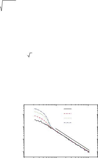
Fig. 6.3: shows form factors obtained for polybutadiene (PB) star polymers with varying functionality f but same Rg 50nm in d-cis-decalin.
|
|
|
f=2 F=3.97· 10-4 |
|
106 |
|
f=6 F=4.58· 10-4 |
/mol] |
|
|
f=16 F=4.95· 10-4 |
5 |
|
f=32 F=3.96· 10-4 |
|
3 |
10 |
|
|
F[cm |
|
|
|
104 |
|
|
|
I(Q)/ |
|
Q-5/3 |
|
|
|
||
|
103 |
|
|
|
-3 |
-2 |
-1 |
|
10 |
10Q [Å-1] |
10 |
Fig. 6.3: SANS intensity I(Q) normalized by volume fraction 055for regular polybutadiene star polymers with varying functionality f but same radius of gyration Rg 50nm. The asymptotic power law observed at high scattering vectors I~Q-5/3 clearly indicates excluded volume interactions relevant in a good solvent , i.e. swollen chain statistics; figure taken from [14].
Macromolecules (structure) |
6.7 |
At low Q-vectors, Q 8×10³ Å1, data could be modelled using the Benoit form factor, Equation (6.2) for a Gaussian star, which gives the explicit dependence on functionality f. For describing the complete data sets we used the Beaucage form factor, Equation (6.3), which describes also the observed power law at high Q-vectors. One should note that this power law extends over more than one order of magnitude in Q and starts at the same Q-value of 8×10³ Å1 for all f due to the same Rg. The observed power law slope of I(Q) ~ Q 5/3 reflects the good solvent quality of cis-decaline for polybutadiene and decreases slightly with increasing f , indicating increasing arm stretching due to the increasing monomer density in the star corona.
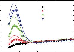
The effect of branching becomes easily visible by using a so called Kratky representation, I(Q) Q2 vs. Q. Whereas a linear polymer with Gaussian chain statistics reaches monotonically an asymptotic plateau, any branched structure shows a maximum. For the here discussed regular star polymer the height quantitatively depends on the arm number or functionality f, see Fig. 6.4:
|
25 |
|
|
|
20 |
|
f=2 F=3.97· 10-4 |
] |
|
f=6 F=4.58· 10-4 |
|
|
|
-4 |
|
2 |
|
|
f=16 F=4.95· 10 |
/Å |
|
|
|
|
|
-4 |
|
15 |
|
f=32 F=3.96· 10 |
|
1 |
|
||
- |
|
|
|
[cm |
|
|
|
|
|
|
|
2 |
10 |
|
|
Q |
|
|
|
F |
|
|
|
I(Q)/ |
5 |
|
|
|
|
|
|
|
0 |
0.01 |
0.02 |
|
0.00 |
||
|
|
Q [Å-1] |
|
Fig. 6.4: Kratky representation I(Q) Q2 vs. Q for same data as in Fig. 6.3. The increasing peak height with increasing functionality f due to branching becomes clearly visible as well as the discrepancy between experimental data (symbols) and Beaucage function used to model the data. The fact that no asymptotic plateau is observed results from the excluded volume interactions relevant in a good solvent, i.e. swollen chain statistics.
6.2.3 In-situ experiments during polymerisation
For understanding and controlling any chemical reaction a detailed understanding of reaction mechanism, type and role of intermediate species as well as reaction kinetics are prerequisite. How the microscopic structure of a growing polymer chain is evolving in the different steps of polymerisation reactions has to be resolved by non-invasive, real-time measurements. The ideal tool is small angle neutron scattering (SANS), since the microscopic structure of polymer-based materials can be resolved on a micrometerto- nanometer-level by modern neutron scattering techniques. In addition, contrast variation, i.e. H/D exchange, can even “stain” certain parts of the polymers giving