Schluesseltech_39 (1)

Fig. 11.4: Brillouin zones for cubic lattices: (a) simple cubic, (b) face-centred cubic, (c) bodycentred cubic. From [10].

The introduction of the quasiparticle (phonon) concept leads to the simple interpretation of inelastic neutron scattering by vibrating lattices: The scattering process can be viewed as a collision between phonons and neutrons. In this process the energy as well as the momentum has to be conserved:

The second equation shows that the analogy with a two-particle collision is not complete. A wave vector, changed by a lattice vector τ in reciprocal space, corresponds to the same phonon. In the one-dimensional case, this can be seen from equation (11.6): If one adds an integer multiple of N to k (corresponding to a multiple of 2π/a in q) all values of the complex exponential remain the same. Analogously, in the three dimensional case adding a lattice vector

does not change anything and momentum has only to be conserved up to an arbitrary reciprocal lattice vector. The condition (11.12) can also be visualised by the Ewald construction as done in lecture 4 for elastic scattering.

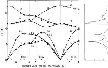
From the conservation laws (11.11) and (11.12) one expects that the scattering intensity has sharp peaks at the positions where both conditions are fulfilled and is zero everywhere else. This is indeed so for coherent scattering, unless effects as multi-phonon scattering and anharmonicity are strong (usually at higher temperatures). Therefore, inelastic scattering allows the straightforward determination of the phonon dispersion relation as shown in Fig. 11.5.

In this figure, it can be seen that some of the phonon ‘branches’ start at the origin (acoustic phonons), as in the simple calculation of the one-dimensional chain. Others are ‘floating’ around high frequencies (optical phonons). The latter occur in materials with atoms of different

[THz]

g( )

Fig. 11.5: Left: Phonon dispersion of NiO measured by inelastic neutron scattering. Frequencies are expressed as ν = ω/2π and the wave vector is expressed in units of ζ = π/a. The lattice is simple cubic, thus the symbols below the abscissa correspond to those in Fig. 11.4(a). Right: Phonon density of states (see section 11.2.3) of NiO plotted to the same scale in frequency. From [11].

weight or bond potential. (The one-dimensional chain would also produce these solutions if the masses were chosen differently for even and odd j.) In this case, a mode, where all atoms of a unit cell move roughly in phase, has the usual behaviour expected from the monatomic chain. In particular the dispersion relation at low q is a proportionality:

This relation is typical for sound waves. v is the sound velocity, longitudinal or transverse according to the type of phonons considered. In the polyatomic crystal or chain, there are additional modes where the atoms move in anti-phase. This implies a much higher deformation of the bonds. These vibrations constitute the optical phonon branches.

There is another difference between the one-dimensional chain and the three-dimensional crystal visible. The atomic displacements are not simply scalars uj but vectors uj which have a direction. This direction can be either parallel or perpendicular to to the wave vector q. Depending on this, one speaks of longitudinal and transverse phonons. The usual notation is LA, TA, LO, TO, where the first letter indicates the phonon polarisation and the second whether it is acoustic or optical. An additional index as T1A is used for q directions where the symmetry allows a distinction between the perpendicular orientations of uj . The full mathematical expression for the phonon scattering [2] includes an intensity factor proportional to |Q · uj |2. This factor obviously vanishes if Q and uj are perpendicular, implying that purely transverse modes are unobservable in the first Brillouin zone where Q = q.

It has to be noted, that the above arguments only hold for coherent neutron scattering (see equation (11.21) below) from crystalline materials. If the material is amorphous the coherent scattering will be diffuse (as it is for incoherent scattering always). The readily understandable reason for this is that the definition of the phonon wave vector q requires a lattice.

Note that this result is independent of the actual structure of the sample. Integration of the double-differential cross section (11.20) over ω shows that also the static scattering contains an incoherent contribution. But because of (11.29), this term is constant in Q. It contributes as a flat background in addition to the S(Q)-dependent scattering. In some cases (e.g. smallangle scattering) it may be necessary to correct for this, in other cases (e.g. diffraction with polarisation analysis) it may even be helpful to normalise the coherent scattering.

In the paragraphs before it was shown, that the value of the intermediate scattering functions at t = 0 corresponds to the integral of the scattering function over an infinite interval. This is a consequence of a general property of the Fourier transform. There is also the inverse relation that the value of S(Q, ω) at ω = 0 is related to the integral of I(Q, t) over all times. The most important case is here when I(Q, t) does not decay to zero for infinite time, but to a finite value f(Q). In that case the integral is infinite, implying that S(Q, ω) has a delta function contribution at ω = 0. This means that the scattering contains a strictly elastic component. Its strength can be calculated by decomposing the intermediate scattering function into a completely decaying part and a constant for the coherent and the incoherent scattering:

Here, t = ∞ indicates a time which is sufficiently long that the correlation with the position at t = 0 is lost. For the EISF this lack of correlation implies that the terms with initial and final

Here, ρj (r) denotes the ‘density of particle j’, i.e. the probability density of the individual par-

ticle j being at r. From (11.34) one can see that the normalisation of the EISF is Sincel (0) = 1 (in contrast to that of the structure factor, limQ→∞ S(Q) = 1). One can say that the EISF is the form

factor of the volume confining the motion of the particles. E.g. for particles performing any kind

of motion within a sphere, the EISF would be Sincel (Q) = 9 (sin(QR) − QR cos(QR))2 /Q6R6 as derived in lecture 5.

As in the static situation, the scattering law can be traced back to distance distribution functions. These are now (in the treatment of inelastic scattering) time-dependent. They are called van Hove correlation functions:

directly proves that the spatial Fourier transforms of the van Hove correlation function are the intermediate scattering functions.

The two particle version can be reduced to the microscopic density,

The 0 is showing that translational symmetry is assumed. So the correlation function can be replaced by its average over all starting points r1 in the sample volume:

In turn this implies that the scattering functions are real and symmetric in energy transfer ω:

It can be seen that this identity violates the principle of detailed balance. Upand downscattering should rather be related by

The reason for this is that (as mentioned in footnote 2) the influence of the neutron’s impact on the motion of the system particles is neglected. This would be included in a full quantummechanical treatment as carried out in ref. 2 or ref. 8 where the detailed balance relation (11.52) emerges in a natural way. Note that equation (11.52) implies that both I(Q, t) and G[s](r, t) are complex functions. (This is not ‘unphysical’ because they are no directly measurable quantities in contrast to S(Q, ω) which is proportional to dσ/dΩdω. Even neutron spin-echo measures only the real part of I(Q, t), see equation (11.69).)

Because the detailed balance relation (11.52) is also valid in classical thermodynamics (and also recoil can be understood in the framework of classical mechanics) there should be a way to derive a correct result from a classical treatment of the system too. This task is important because only rather simple systems can be treated quantum-mechanically. Especially, results from molecular dynamics computer simulations are classical results. The result for S(Q, ω) derived here is obviously only a crude approximation. Better approximations can be obtained by applying correction factors restoring (11.52) [16–18]. The exact classical calculation is rather complicated [19] and requires knowledge of the system beyond just the trajectories of the particles.

Inelastic scattering is often also called neutron (scattering) spectroscopy. That there is indeed a relation to better-known spectroscopic methods as light spectroscopy, can be seen from the dependence of the scattering function on a frequency ω. It can be said that inelastic neutron scattering, for every Q, produces a spectrum, understood as the frequency dependence of a quantity, here the scattering cross section. The optical methods Ramanand Brillouin spectroscopy are completely analogous in this respect, yielding the same S(Q, ω) but different measured doubledifferential cross-sections because photons interact with matter differently. Other methods, as absorption spectroscopy, impedance spectroscopy or rheology do not yield a Q dependence and are thus insensitive to the molecular structure. They provide only information about the overall dynamics. The deeper reason for this analogy is that scattering experiments as well as ‘ordinary’ spectroscopy can be explained by linear response theory (appendix B of ref. 2 or ref. 15).

Example: diffusion

For simple diffusion the density develops in time following Fick’s second law,

The underlying mechanism is Brownian motion, i.e. random collisions with solvent molecules. Therefore, it can be concluded from the central limit theorem of statistics that the density of

particles initially assembled at the origin is a Gaussian in all coordinates:

The index 1 should remind that the prefactor is chosen such that the total particle number

ρ1 d3r is normalised to one. The width of the distribution, σ has the dimension length.

√

The only way to construct a length out of D (dimension length2/time) and time is σ = c Dt where c is a dimensionless constant. Inserting this into (11.54) yields:

The derivatives of this expression with respect to t and x, y, z can be calculated and inserted into (11.53):

√

One can see that the rightand left-hand side are identical if c = 2. This proves that the ‘guess’ (11.54) is indeed a solution of Fick’s second law and also determines the unknown c. With the value of c substituted, the ‘single particle density’ is

Diffusion-like processes are often characterised by the mean-square displacement r2 5. Because of the statistical isotropy, the average displacement r is always zero. Therefore, the characterisation of the mobility of a diffusional process has to be done using the second moment, which is the average of the square of the displacement. For the simple Fickian diffusion this can be calculated from (11.57):

r2 = ρ1r24πr2d3r = 6Dt . (11.58)

For incoherent scattering the starting position r(0) is irrelevant. Therefore, expression (11.57) is also Gs(r, t). Because the Fourier transform of a Gaussian function is a Gaussian itself, the corresponding incoherent intermediate scattering function is

5 Here, the definition is “displacement from the position at t = 0” rather than “displacement from a potential minimum” on page 8. This is an obvious choice because the diffusing particle is not subjected to a potential as the atom in a crystal. Therefore, there is nothing like an ‘equilibrium position’. This difference is indicated by the usage of r2 instead of u2 . Because in the case of motion in a potential the displacement between time zero and time t can be understood as the difference of the displacements at time zero from the equilibrium position and that at time t, it follows that r2 = 2 u2