Schluesseltech_39 (1)

access to unprecedented structural information. So neutron scattering is a unique and outstanding technique to investigate polymerising systems in real-time, in particular since new, more powerful neutron sources became available worldwide (FRM-2, SNS, J-PARC). But for a complete description of the polymerisation process additional information in terms of reaction kinetics etc. are prerequisite. Thus, in-situ SANS experiments have to be supported by complementary methods like NMR, SEC, UV/VIS and IR spectroscopy, favourably also in real-time mode.

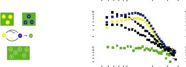
Recently we investigated reaction mechanism and kinetics of different polymerisation techniques like “living” anionic polymerisation [15] or post-metallocene catalyzed olefin polymerisation [16] by such an in-situ multi technique approach. Fig. 6.5: shows time resolved SANS intensities I(Q) in absolute units obtained during the polymerisation of 1-octene by a pyridylamidohafnium catalyst in toluene at 20°C. Experiments have been performed using the KWS-1 instruments at the former FRJ-2 reactor in Jülich which allowed a temporal resolution of about several minutes.

Fig. 6.5:Time resolved SANS intensities I(Q) in absolute units obtained during the polymerisation of 1-octene by a pyridylamidohafnium catalyst in toluene at 20°C; figure taken from [16].

Whereas the monomer solution shows a Q-independent intensity over the whole accessible SANS Q-range typical for small molecules (“incoherent scatterers”), after 4 minutes a polymer is already formed and the Q-dependence of the intensity can be described by a Beaucage form factor, Equation (6.3). With ongoing polymerisation, increasing polymerisation time t the general shape of I(Q) does not change any further, only the forward scattering I(Q=0) is increasing due to the increasing molecular weight and concentration of the growing polymer chain. Finally, the polymerisation is almost finished after half an hour as can be seen by comparison with the terminated polymer. A detailed quantitative analysis of I(Q,t) reveals that during this type of polymerisation reaction no aggregation phenomena of the growing polymer chain are relevant. Similar experiments at high flux sources allow today temporal resolutions smaller than 1 second if experiments are repetitively performed using a stopped flow mixer.

6.3 Block copolymer Micelles

When amphiphilic block copolymers are dissolved in a selective solvent, i.e. a solvent which is good for one block but a precipitant for the other, they spontaneously selfassemble into supramolecular aggregates known as micelles, in which the insoluble block forms the inner part or core, whereas the soluble block forms a solvent-rich shell or corona. The general behaviour of block copolymers in selective solvents has been subject of copious theoretical and experimental studies during the past decades. They are reviewed in several books [17] [18] and review articles [19][20] related to this topic. Extensive studies demonstrated that the micellar morphology can be tuned (going from spheres, cylinders, worms and vesicles) by varying the block-copolymer molecular weight, the chemical nature and the ratio of the blocks. One of the most extensively studied block-copolymers is poly(butadiene-ethylene oxide) (PB-PEO). As a function of the hydrophilic block length (in term of PEO weight fraction wPEO) spherical micelles (wPEO >0.6), worm-like micelles, WLM (0.47 KwPEO K 0.59) or bilayers (wPEO <0.47) are formed. Different theoretical studies contributed to define the scaling laws for the parameters of equilibrium structures. Among them, a quantitative theory defining the thermodynamic stability of different morphologies in selective solvents has been recently developed [21]. The theory expresses the free energy contributions of the core, the corona and the interface as a function of the blocks structural parameters and the interfacial tension between the solvent and the insoluble block for different micellar morphologies. Solvent selectivity can be more easily tuned than the above mentioned parameters (molecular weight, block ratio etc) and moreover in a continuous way by varying the solvent composition. Therefore solvent composition is a very natural and easy parameter to control the micellar structures. The change in the morphology of the self-assembled structures can be attributed to a change of solvent selectivity, which influences the different energy contributions responsible for the morphology: core-chain stretching, corona-chain repulsion and interfacial tension between the core and the solution.

The interest is to relate changes on the smallest relevant length scale, i.e. diameter and aggregation number per unit length, density profile in the corona, to changes in the macroscopic structure, i.e. the contour and persistence length of wormlike micelles and the transition from wormlike-to-spherical micelles etc. This molecular level understanding can help to elucidate the mechanisms involved in non equilibrium conditions. Besides, it is expected that these quantities have a pronounced effect on the rheological behavior of the systems, and as such solvent composition could be used to tune the flow properties of micellar solutions.

6.3.1 Form factor

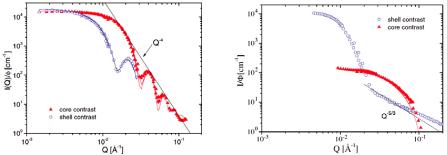
Figure 6.6 (left) shows the partial form factor normalized to volume fraction , P(Q)/ , in shell and core contrast for micelles formed by a symmetric amphiphilic block copolymer poly(ethylene-alt-propylene)–poly(ethylene oxide), h-PEP4-dh-PEO4 (the numbers denote the block molecular weight in kg/mol) [22]. Already, a qualitative discussion of the data reveals important features of the micellar architecture. First, the forward scatterings, I (Q = 0), in the two contrasts are the same. This is expected for micelles formed by a symmetric diblock copolymer in shell and core contrast (we should note that the two blocks have the same molar volume Vw) and is in this sense a

proof of the applied contrast conditions. This means that the scattering profiles shown in figure 2 are directly reflecting pure shell and core properties. Second, both scattering profiles show well defined maxima and minima, up to 4 in core contrast, which arise from sharp interfaces typical for a monodisperse, compact particle. Also shown is

Porod’s law I Q 4, which describes the limiting envelope of all form factor

oscillations. (We should note that one has to consider that these oscillations are already smeared by the instrumental resolution function, so the data shown offer even more confirmation of the strong segregation between the core and corona and the low polydispersity of the micelles.) We should emphasize that in core contrast no blob scattering is visible [22]. This also corroborates the compact PEP core. A quantitative analysis in terms of a core–shell model gave the following micellar parameters: aggregation number P = 1600, core radius Rcore = 145 Å and shell radius Rm = 280 Å with a polydispersity of 5%. The solvent fraction in the swollen shell is solv = 60%.

Figure 6.6 (right) shows the corresponding partial form factor data, P(Q)/ , in shell and core contrast for an asymmetric h-PEP1-dh-PEO20. The differences compared to figure 6.6. (left) are obvious: the difference in forward scattering of the two contrasts is reflecting the asymmetry of the block copolymer. Moreover, no maxima or minima are visible (also not at high Q in core contrast) and the power law observed in shell contrast

has a slope of only I Q 5/3, which is typical for a polymer chain in a good solvent and

arises from the swelling of the PEO in the shell (blob scattering). A quantitative analysis gives the following micellar parameters: aggregation number P = 130, core radius Rcore = 34 Å and shell radius Rm = 260 Å.

Fig. 6.6:Form factors of block copolymer micelles with varying architecture in core (red) and shell contrast(blue). Left symmetric PEP4-PEO;right asymmetric PEP1-PEO20, the numbers denote the block molecular weight in kg/mole. Figure taken from [22].

6.3.2 Micellar exchange dynamics

Polymeric micelles are macromolecular analogues of well-known low-molecular surfactant micelles. As a consequence of random stochastic forces, the constituting chains will continuously exchange between the micelles. From the theory of Halperin and Alexander (HA), this exchange kinetics is expected to be dominated by a simple expulsion or insertion mechanism where single chains (unimers) are required to overcome a defined potential barrier [23]. Higher order kinetics including fusion and

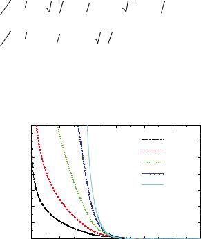
fission is not expected to take place since these mechanisms are neither favored energetically nor entropically [24]. Experimentally, relatively few studies have been devoted to the exchange kinetics of polymeric micelles in equilibrium. This is most likely related to the associated experimental difficulties. Recently, we used a newly developed time resolved small angle neutron scattering (TR-SANS) technique [25]. This technique is perfectly suited for determination of exchange kinetics in equilibrium as, unlike other techniques; virtually no chemical or physical perturbations are imposed on the system. The labeling is restricted to a simple hydrogen/deuterium (H=D) substitution using fully hydrogenated (h) and fully deuterated (d) polymers with identical molar volumes and compositions. By mixing the corresponding H- and D-type micelles in a solvent with a scattering length corresponding to the average between the two, the kinetics can be determined. The average excess fraction of labeled chains residing inside the micelles is then simply proportional to the square root of the excess SANS intensity. The corresponding correlation function is given by

R(t) QGI(t) I H/GI(t 0) I HR1/ 2 was measured from a reference sample where the polymers have been completely randomized and I(t=0) from the scattering of the reservoirs at low concentrations.

Fig. 6.7:Left: Schematic illustration of the TR-SANS technique to follow micellar exchange kinetics. Right: Corresponding time-resolved SANS data forPEP1PEO20 micelles in H2O/DMF 7:3 showing slow exchange (5min, 2h @ 50°C).

6.3.3 Structure factor

How the structure factor S(Q) can be derived from the pair correlation function g(r) by liquid state theory has been shown in Chapter 5.3.4. g(r) finally results from the effective pair potential V(r), which describes the direct interactions between the solute only, after eliminating the rapidly moving degrees of freedom of the solvent molecules. We recently showed that micelles formed by the amphiphilic block copolymer poly(ethylene-alt-propylene)– poly(ethylene oxide) (PEP–PEO) provide an interesting system to conveniently tune the ‘softness’ in terms of particle interactions (intermolecular softness) and the deformability of the individual particle (intramolecular softness). This is achieved by changing the ratio between hydrophobic and hydrophilic blocks from symmetric (1:1, Hard Sphere-like) to very asymmetric (1:20, star-like). One must emphasize that to approach the star-like regime is not a trivial task.

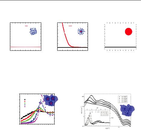
Figure 6.6 compares the effective interaction potential for soft colloids to those of the limiting cases Gaussian Chain, i.e. no interactions, and Hard Spheres, i.e. infinite strength of the potential at contact. The explicit form of V(r) for star polymers, the

limiting ultra-soft colloids, was derived by Likos et al. [26] and is explained in detail in Appendix 6.1.

Fig. 6.8:Different effective interaction potentials. The one for star polymers, i.e. soft colloids, is in-between the two limits Gaussian Chain (left) and Hard Spheres (right).

Figure 6.9 shows the corresponding experimental structure factors S(Q) for Hard Sphere and Soft interactions and its comparison with theoretical predictions.

Fig. 6.9:Experimental structure factor S(Q) of block copolymer micelles with varying architecture obtained by SANS in core contrast (symbols) and the theoretical description (lines) resulting from the corresponding interaction potentials: Symmetric PEP4-PEO4 / Hard Sphere potential left, asymmetric PEP1PEO20/ ultra soft potential right, see text and [22].

6.4 Soft Colloids

Soft colloids in general, e.g. polymer-coated silica particles, block copolymer micelles, star polymers etc., are hybrids between (linear) polymer chains and (hard sphere) colloids. Due to this hybrid nature, soft colloids macroscopically show interesting (phase) behaviour resulting from its unique microscopic structure. The combination of polymer-like properties, i.e. the formation of (transient) geometric constraints due to overlapping polymeric coronas and direct colloidal interactions due to the (hard) core in particular affects flow properties and nonequilibrium behaviour of soft colloids. Therefore soft colloids are frequently used in many technical applications (paints, shampoos, motor oils, polymer nano-composites etc.).

More recently, the interest of colloid scientists in fundamental science has shifted towards the study of soft particles, among which star polymers have emerged as a

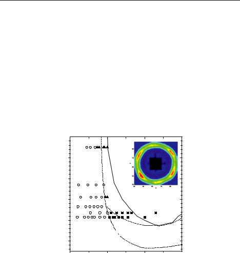
model system for a wide class of soft spheres. For a star polymer, softness can be controlled by varying its number of arms (or functionality f), allowing to bridge the gap between linear polymer Gaussian chains (f = 2) and Hard Spheres (f = ). Therefore, star polymers feature tuneable softness, which is responsible for the observation of anomalous structural behaviour and for the formation of several crystal structures [28]. Hence, mixtures of soft particles offer an even higher versatility with respect to their hard counterparts, both in terms of structural and rheological properties and of effective interactions. Recently, we confirmed experimentally by combining SANS and rheology the theoretical phase diagram of soft colloids [29] and mixtures of soft colloids with linear polymers [29]. As experimental realization again the previously described PEPPEO star-like micelles have been used. Figure 6.10 shows the phase diagram in the functionality vs. packing fraction representation. We have to point out that quantitative agreement starting from experimental parameters is achieved without any adjustable parameter. For this the determination of the interaction length by SANS in core contrast was inevitable.

Fig. 6.10: Phase diagram of ultra soft colloids (symbols experiment: fluid, bccamorphous solid;, lines theory). Figure taken from.

References

[1]C J.R. Severn and J.C. Chadwick, Tailor-Made Polymers, (Wiley-VCH, Weinheim, 2008)

[2]G.W. Coates and M.A. Hillmyer, Polymers from Renewable Resources, Macromolecules, VI2, 7987 (2009); C.K. Williams, M.A. Hillmyer, Polymer Rev. 48, 1 (2008)

[3]J. S. Higgins and H. C. Benoit, Polymers and Neutron Scattering; (Clarendon Press, Oxford, U.K., 1994).

[4]P.G. De Gennes, Scaling Concepts in Polymer Physics, (Cornell University Press, 1979)

[5]W. Brown, Light Scattering: Principles and development, (Oxford University Press, 1996)

[6]S. Mori and H.G. Barth, Size Exclusion Chromatography, (Springer, 1999)

[7]P.J. Flory, Principles of Polymer Chemistry, (Cornell University Press, 1953)

[8]H.G. Elias, Macromolecules, (Wiley-VCH, Weinheim, 2009)

[9]G. S. Grest, L. J. Fetters, J. S. Huang, and D. Richter, Adv. Chem. Phys. 94, 67 (1996)

[10]J. Allgaier, K. Martin, H. J. Räder, and K. Müllen, Macromolecules 32, 3190 (1999)

[11]H.J. Benoît, J. Polym. Sci., 11, 507 (1953).

[12]William D. Dozier, John S. Huang, Lewis J. Fetters, Macromolecules 24 2810 (1991)

[13]G. Beaucage, J. Appl. Crystallogr. 28, 717(1995)

[14]J. Stellbrink et al., Applied Physics A 74, S355 (2002)

[15]J. Stellbrink et al. Macromolecules, 31, 4189 (1998)

[16]A.Z. Niu et al., Macromolecules 42 1083 (2009)

[17]I.W. Hamley, The Physics of Block Copolymers; (Oxford University Press: New York, 1998)

[18]M. Antonietti and S. Förster, Vesicles and Liposomes: A Self-Assembly Principle Beyond Lipids, Vol. 15, (WILEY-VCH Weinheim, , 2003)

[19]G. Riess, Prog. Polym. Sci. 28, 1107 (2003)

[20]A. Halperin, M. Tirell and T.P. Lodge, Adv. Polym. Sci. 100, p31 (1990).

[21]E.B. Zhulina, M. Adam, I. LaRue, S.S. Sheiko, M. Rubinstein, Macromolecules 38, 5330 (2005)

[22]J. Stellbrink, G. Rother, M. Laurati, R. Lund, L. Willner and D. Richter, J. Phys.: Cond. Matter, 16, S3821 (2004)

[23]A. Halperin and S. Alexander, Macromolecules 22, 2403 (1989)

[24]E. Dormidontova, Macromolecules 32, 7630 (1999)

[25]L. Willner, A. Poppe, J. Allgaier, M. Monkenbusch, and D. Richter, Europhys. Lett. 55, 667 (2001)

[26]C.N. Likos et al., Phys. Rev. Letters, 80, 4450, (1998)

[27]M. Watzlawek, C. N. Likos, and H. Lowen, Phys. Rev. Lett. 82, 5289 (1999).

[28]M. Laurati, Phys. Rev. Letters, 94 195504 (2005)

[29]B. Lonetti et al. Phys. Rev. Letters, 106, 228301 (2011)

Exercises

E6.1 Contrast or no contrast?

Due to synthetic (and financial) limitations only protonated material is available for a SANS experiment, for both polymer (poly(ethylene propylene), PEP, and solvent dimethylformamide, DMF.

a) Calculate the contrast factor E 2 .

NA

b)What is the necessary molecular weight Mw to achieve a signal-to-background ratio of 5 at Q=0 for a given polymer volume fraction 0p =0.01? (Remember: Also the incoherent scattering contributes to the background and there is an empirical “rule of thumb” that the experimental incoherent scattering is twice the theoretical value due to inelastic and multiple scattering!)

c)At which Q-value the signal vanishes in the background?

(Assuming good-solvent conditions with a prefactor 0.01 [nm] for the Rg-Mw-relation and assuming the Guinier approximation for P(Q))

d) For which combination of molecular weight and volume fraction 0p the experiment could be performed in the dilute regime, i.e. 0p 0.10*?

Given are sum formulae and densities

h-PEP = C5H10, dPEP=0.84g/cm3

h-DMF = C3H7NO, dPEO=0.95g/cm3

and coherent and incoherent scattering lengths bcoh and binc in units [cm]:

E6.2 Contrast factors for Micelles

In aqueous solution, the diblock copolymer poly(ethylene propylene-block-ethylene oxide), PEP-PEO, forms spherical micelles, with PEP the non-soluble and PEO the soluble block. Using SANS combined with contrast variation the micellar structure should be investigated. To prepare the corresponding samples the following parameters have to be calculated

a.) the coherent scattering length densities PEP and PEO in units of [cm-2]:

Known are the monomer sum formulae and densities h-PEP = C5H10, dPEP=0.84g/cm3

h-PEO = C2H4O, dPEO=1.12g/cm3

the degree of polymerisation, Dp, of the blocks:

Dp,PEP = 15

Dp,PEO = 40

and the coherent scattering lengths bcoh in units [cm]: C=6.65E-13

H=-3.741E-13

D=6.671E-13

O=5.803E-13

b.) the isotopic solvent mixture (H2O/D2O) that match the scattering length density of either PEP and PEO.

Given: dD2O=1.1g/cm3

E6.3 Aggregation number of micelles

For the same PEP-PEO micelles as in E6.2, in dilute solution using core contrast, i.e. the scattering length density of the solvent is matched to the scattering length density of the micellar shell (formed by the soluble block PEO), the first form factor minimum is observed at Q=0.12 Å-1.

Calculate

a.) the aggregation number Nagg, i.e. the number of diblock copolymers forming a single micelle, assuming full segregation, i.e. a non-swollen micellar core.

b.) How can Nagg derived in this way be cross-checked without performing another experiment?

E6.4 Reduced forward scattering (virial expansion)

For the same PEP-PEO micelles as in E6.2 at finite concentration using core contrast the corresponding forward scattering I(Q=0) for volume fractions 01=1x10-3, 02=5x10-3 and 03=7.5x10-3 assuming a second virial coefficient A2=2x10-4 should be calculated.

E6.5 Peak position in S(Q)

A solution of compact spherical colloids, R=250Å, with volume fraction 0.25 should be characterised by SANS. At which Q-vector do you expect the first peak in the structure factor S(Q) to appear?