Schluesseltech_39 (1)

4.1 Introduction

Each scattering experiment performed with any type of radiation - regardless of whether it involves massive particles like neutrons and electrons or electromagnetic waves like x-rays or visible light - has a total of four attributes which altogether characterize the type of the scattering experiment as well as the information that can be obtained from such an experiment. These attributes and their characteristics are:

Elastic scattering, which involves the conservation of the energy of the particle or quantum during the scattering process, inelastic scattering, corresponding to a loss or gain of particle or quantum energy during the scattering event, coherent scattering which involves the interference of waves (recall that, according to the particle-wave dualism first stated by de Broglie (1924), each particle may also be described by wave which can interfere with other particle waves) and finally incoherent scattering which is scattering without interference.

Fig. 4.1: Scattering function S(Q,@) of a general scattering experiment (Q: scattering vector, @: frequency), its different contributions and information that can be obtained from them.

This chapter will deal mostly with neutron diffraction which is, in the above nomenclature of a general scattering experiment, equivalent to elastic coherent scattering of neutrons.

Most of the readers of this chapter will be more or less familiar with x-ray diffraction from crystals, which has been demonstrated for the first time by Laue in 1912 and, since then, has developed into the most powerful method for obtaining structural information on crystalline materials. Diffraction - in sharp contrast to imaging techniques like optical or electron microscopy - has no principal limitation as to the spatial resolution, expressed in units of the wavelength of the radiation used for diffraction or imaging: While the resolution of imaging is limited to half the wavelength (recall the Abbe diffraction limit) diffraction can yield useful information, for instance, on bond distances between atoms on a length scale that is by two to three orders of magnitude smaller than the wavelength. On the other hand, diffraction, other than imaging,

requires 3-dimensional periodicity that is underlying the concept of the crystalline state (see chapter 3, symmetry in crystals).

This chapter will discuss the basics and peculiarities of neutron diffraction from either singleor polycrystalline matter. We will start by discussing scattering of neutrons from individual atoms, then turn to the geometry of diffraction from crystals, treat the subject of diffraction intensities and end with a discussion of a few experimental issues connected to the instruments which will be used in the practical part of the course. Examples of applications of these methods will be given in chapter 8 “structural analysis”. The subject of magnetic neutron diffraction and scattering will be discussed separately in chapter 7.

4.2 Neutron waves & neutron scattering

The three major probes for investigating condensed matter are photons, electrons and neutrons. While photons are the (massless) quanta of electromagnetic radiation (e.g. x- rays, including synchrotron radiation, but also visible light, gamma-rays etc.) electrons and neutrons are massive particles. Owing to the wave-particle-duality, a central concept of quantum mechanics that states that all particles exhibit both waveand particle-properties, the formal description of a scattering experiment does not differ for these different probes. However, the relation between energy and wavelength of the probes and also the mechanisms by which they interact with matter are vastly different.

Fig. 4.2: Comparison of the three probes - neutrons, electrons and photons - in a double logarithmic energy-wavelength diagram. Added to the figure are the typical size of objects to be studied and the energy of thermal neutrons.

As the horizontal line at a wavelength of 1 Å shows, neutrons of this wavelength have an energy as low as about 80 meV, while 1 Å electrons correspond to about 150 eV and 1 Å photons (x-rays) have energies in excess of 12 keV. All three types of radiation

with this wavelength are well suited for scattering experiments on objects like atoms, molecules and crystals. The investigation (by scattering) of larger objects like colloids (in the 100 nm size range) requires, correspondingly, much lower energy probes like, for instance, photons in the ultraviolet range (about 12 eV).

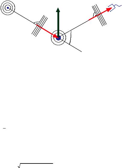
The scattering process

detector

source

Fig. 4.3: Sketch of the scattering process with the incoming wave characterized by wavevector k, diffracted wave by k' and the sample by scattering vector Q, assumed: plane waves, (Fraunhofer approximation, source-sample and sample-detector distances much larger than sample size), also assumed: monochromatic radiation (single wavelength)

k is also called the wave number of the neutron and is conserved during scattering because the neutron energy and therefore the wavelength does not change.

The units of k, k’ and Q are Å-1.

Q represents the momentum transfer during scattering, since according to de Broglie, the momentum of the particle corresponding to the wave with wave vector k is given by p= k. The magnitude of the scattering vector can be calculated from wavelength B and scattering angle 2 as follows

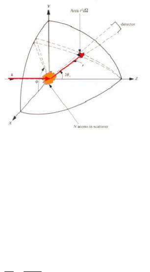
A scattering experiment comprises the measurement of the intensity distribution as a function of the scattering vector I(Q). The scattered intensity is proportional to the so-

called cross section, where the proportionality factors arise from the detailed geometry of the experiment. For a definition of the scattering cross section see Figure 4.4.

Fig. 4.4: Geometry used for the definition of the scattering cross section.

This is in close analogy to the absorption cross section derived in chapter 2.

Let us drop, for a moment, the assumption of strictly elastic scattering and treat the universal case of a general scattering experiment (will be needed in other chapters):

If n' particles are scattered per second into the solid angle d. seen by the detector under the scattering angle 2 and into the energy interval between E' and E' + dE', then we can define the so-called double differential cross section by:

Here j refers to the incident beam flux in terms of particles per area and time. If we are not interested in the change of the energy of the radiation during the scattering process, or if our detector is not able to resolve this energy change, then we will describe the angular dependence by the so-called differential cross section:

dD d2D dE ' (4.5) d. 0 d.dE '

Finally the so-called total scattering cross section gives us a measure for the total scattering probability independent of changes in energy and scattering angle:

All the information about the scattering matter is contained in the (double differential) scattering cross section. This includes positions and possible motions of scatterers in the

sample volume. Note that in most diffraction experiments (with x-rays in particular, but also with electrons and neutrons), the actual measurement is energy-integrated because the detectors used are energy-insensitive. Consequently, the inelastic scattering also contributes to the measured intensity, but it is usually much weaker than the purely elastic scattering. Neutron scattering, however, offers the unique opportunity to set a very narrow energy window and study purely elastic scattering as well as inelastic scattering at arbitrary energies.

If we go back to elastic scattering the information on the positions of the scatterers is contained in the differential cross sectiondD / d. . The relationship between scattered intensity and the structure of the sample is particularly simple in the so-called Born approximation, which is often also referred to as kinematic scattering approximation. In this case, refraction of the beam entering and leaving the sample, multiple scattering events and the extinction of the primary beam due to scattering within the sample are being neglected. According to Figure 4.5, the phase difference between a wave scattered at the origin of the coordinate system and at position r is given by

EF 2 AB CD k ' r k r Q r (4.7)

B

no refraction

no attenuation

vs

single scattering event

Fig. 4.5: Elastic scattering from a non-periodic object, illustrating the phase difference between a beam scattered at the origin of the coordinate system (A) and a beam scattered at the position r. Additional caption: underlying assumptions of the kinematic scattering approximation.

The scattered amplitude at position r is proportional to the scattering density s(r) at this position. s depends on the type of radiation used and the interaction of this radiation with the sample. In fact, s is directly proportional to the interaction potential, as will be shown in the next paragraph. Assuming a laterally coherent beam, the total scattering amplitude is given by a coherent superposition of the scattering from all points within the sample, i. e. by the integral

Here A0 denotes the amplitude of the incident wave field. (4.8) demonstrates that the scattered amplitude is connected with the scattering density s(r) by a simple Fourier

transform. Knowledge of the scattering amplitude for all scattering vectors Q allows us to determine via a Fourier transform the scattering density uniquely. This is the complete information on the sample, which can be obtained by the scattering experiment. Unfortunately, nature is not so simple. On one hand, there is the technical problem that one is unable to determine the scattering cross section for all values of momentum transfer Q. The more fundamental problem, however, is that normally the amplitude of the scattered wave is not measurable. Instead only the scattered intensity

I ~ A 2 (4.9)

can be determined. Therefore the phase information is lost and the simple reconstruction of the scattering density via a reverse Fourier transform is no longer possible. This is the so-called phase problem of scattering. There are ways to overcome the phase problem, either experimentally, e. g. by use of reference waves (holography) or by using a priori information about the scattering density function (like positiveness or peakedness) which is the basis of the so called direct methods of structure determination that is very frequently used in x-ray crystallography. The question, which information we can obtain from a conventional scattering experiment despite the phase problem will be addressed below.

Which wavelength do we have to choose to obtain the required real space resolution? For information on a length scale L, a phase difference of about Q L 2 has to be achieved. Otherwise k' and k will not differ significantly (see eqn. (4.7)). According to (4.3) Q 2 /B for typical scattering angles (2 ~ 60°). Combining these two estimates, we end up with the requirement that the wavelength B has to be on the order of the real space length scale L under investigation. To give an example: with the wavelength in the order of 0.1 nm, atomic resolution can be achieved in a scattering experiment.

Coherence

In the above derivation, we assumed plane waves as initial and final states. For a real scattering experiment, this is an unphysical assumption. In the incident beam, a wave packet is produced by collimation (defining the direction of the beam) and monochromatization (defining the wavelength of the incident beam). Neither the direction kˆ , nor the wavelength B have discrete values but rather have a distribution of non-vanishing width about their respective mean values. This wave packet can be described as a superposition of plane waves. As a consequence, the diffraction pattern will be a superposition of patterns for different incident wavevectors k and the question arises, which information is lost due to these non-ideal conditions. This instrumental resolution is intimately connected with the coherence of the beam. Coherence is needed, so that the interference pattern is not significantly destroyed. Coherence requires a phase relationship between the different components of the beam. Two types of coherence can be distinguished:

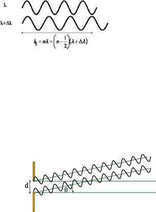
Temporal or longitudinal coherence due to a wavelength spread:

A measure for the longitudinal coherence is given by the length, on which two components of the beam with largest wavelength difference (B and B+EB) become fully out of phase.

Fig. 4.6: Sketch illustrating the longitudinal coherence due to a wavelength spread.

From this, we obtain the longitudinal coherence length l|| as

Transverse coherence due to source extension:

Due to the extension of the source (transverse beam size), the phase relation is destroyed for large source size or large divergence. According to the following figure, a

first minimum occurs for B d sin d .

2

Fig. 4.7: Sketch illustrating the transverse coherence due to source extension and beam divergence.

Here E is the divergence of the beam. Note that l< can be different along different

spatial directions: in many instruments, the vertical and horizontal collimations are different.

Together, the longitudinal and the two transversal coherence lengths (in two directions perpendicular to the beam propagation) define a coherence volume. This is a measure for a volume within the sample, in which the amplitudes of all scattered waves superimpose to produce an interference pattern. Normally, the coherence volume is

significantly smaller than the sample size, typically a few 100 Å for neutron scattering, up to μm for synchrotron radiation. Scattering between different coherence volumes within the sample is no longer coherent, i. e. instead of the amplitudes the intensities of the contributions to the scattering pattern have to be summed up. This limits the real space resolution of a scattering experiment to the extension of the coherence volume.

Neutron scattering from atomic nuclei

Neutrons interact with the nuclei of the atoms by potential scattering as well as with the magnetic moment of unpaired electrons in the electron shells of the atoms. Here we focus on the so-called nuclear scattering contribution. As the wavelength of thermal neutrons (approx. 10-10 m) is much larger than the diameter of the atomic nucleus (10-14

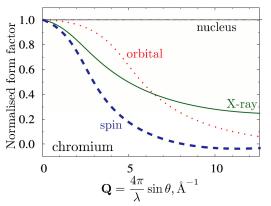
...10-15 m), the atom is essentially a point scatterer. As the construction of Fig. 4.5 and equation (4.7) shows, this means that the length of the vector r (now a vector within the nucleus) is very small compared to the wavelength of the neutron and therefore the phase difference of waves from different parts of the nucleus is essentially zero. This is in sharp contrast to x-ray diffraction, where the scattering occurs from the electron cloud and the size of the scatterer and the wavelength of the radiation are similar. This results in the well-known formfactor falloff of the scattered intensity with increasing scattering angle. The same holds true for the magnetic formfactor for thermal neutrons. Magnetic neutron scattering will be the subject of chapter 7. For neutron scattering from the atomic nuclei, the formfactor is a constant. This is one big advantage of neutrons over x-rays because there is still an appreciable amount of scattered intensity even at very high scattering angles, where an x-ray experiment will yield hardly any useful information.

Fig. 4.8: Form-factor of Cr [1]. On the Å length scale of the thermal neutron wavelength, the nucleus is point-like, therefore, nuclear scattering is independent of the scattering angle. For x-rays and magnetic neutron scattering, the form factor falls off with increasing scattering angle. For more details on magnetic neutron scattering see chapter 7.

The interaction that governs nuclear neutron scattering (essentially potential scattering) is the strong nuclear force. Note that, despite the fact that the strong interaction of high

energy physics is responsible for the scattering of the neutron with the nucleus, the scattering probability is very small due to the small nuclear radius.

The quantity that describes the interaction between neutrons and matter is the scattering length b, it is usually expressed in units of a Fermi (1 fm = 10-15 m). Another frequently

used quantity is the total cross section of a given nucleus D 4 b 2 corresponding to

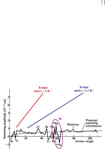
the surface area of a sphere with radius b. D is usually expressed in barns, 1 barn = 10-24 cm2. A simple description of potential scattering predicts the smooth increase of the scattering length with increasing atomic weight depicted in Figure 4.9 by the dashed line. Obviously, this description is rather crude as resonance effects play an important role and, consequently, there are pronounced deviations from this line. As the interaction potential depends on the details of the nuclear structure, scattering lengths b can be very much different for different isotopes of the same element and also for different nuclear spin states (see chapter 7). In fact, neutron nuclear scattering lengths are still very hard to calculate (in contrast to x-ray scattering where the scattering power of any atom can be calculated to a very high precision) illustrating our still quite limited knowledge of the nuclear structure of atoms as opposed to the very well understood electronic structure of atoms. Consequently, the tabulated values of b which can be found in [2] or at http://www.ncnr.nist.gov/resources/n-lengths/ are experimentally measured quantities, not calculated ones. The scattering length is mostly positive but can also adopt negative values, this negative sign corresponds to a phase shift of (or 180°) during the scattering process. The fact that different isotopes of the same element have different scatterings lengths also gives rise to the appearance of so-called incoherent scattering (see below).

Fig. 4.9: Scattering length as a function of atomic weight throughout the periodic table (from Research, London 7 (1954), 257). Note the two different curves for x- rays at lowand high scattering angles, illustrating the formfactor falloff that is typical for x-rays but doesn’t exist for nuclear neutron scattering.

In Figure 4.10, the scattering cross sections for x-rays and neutrons are compared. Note that the x-ray scattering cross sections are in general a factor of 10 larger as compared to the neutron scattering cross sections. This means that the signal for x-ray scattering is stronger for the same incident flux and sample size. For x-rays, the

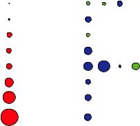
cross section depends on the number of electrons and thus varies in a monotonic fashion throughout the periodic table. Clearly it will be difficult to determine hydrogen positions with x-rays in the presence of heavy elements such as metal ions. Moreover, there is a very weak contrast between neighboring elements as can be seen for the transition metals Mn, Fe and Ni in Figure 4.10. However, this contrast can be enhanced by anomalous scattering, if the photon energy is tuned close to the absorption edge of an element. For neutrons the cross section depends on the details of the nuclear structure and thus varies in a non-systematic fashion throughout the periodic table. As an example, there is a very high contrast between Mn and Fe. With neutrons, the hydrogen atom is clearly visible even in the presence of such heavy elements as Uranium. Moreover there is a strong contrast between the two Hydrogen isotopes H and D. This fact can be exploited for soft condensed matter investigations by selective deuteration of certain molecules or functional groups. This will vary the contrast within the sample.

0.66 H 1.76

24 C 5.55

6

416 Mn1.75

25

450 Fe 11.22

26

522 Ni 13.30

28

58 60 62

1408 Pd4.39

46

2986 Ho8.06

67

5631 U 8.90

92

x-ray element neutrons

Z

Fig. 4.10: Comparison of the (coherent) scattering cross-sections for x-rays and neutrons for a selection of elements. The area of the colored circles represent the scattering cross section, where in the case of x-rays a scale factor 10 has to be applied. For neutrons, the blue and green circles distinguish the cases where the scattering occurs with or without a phase shift of . For 1H and 28Ni, scattering cross sections for certain isotopes are given in addition to the averaged values for the natural abundances.

Coherent and incoherent scattering

As mentioned above, the scattering length b is different for different isotopes of a given element and also for different nuclear spin states. This gives rise to an additional contribution to the total intensity, the incoherent scattering. In this chapter, we will