Schluesseltech_39 (1)

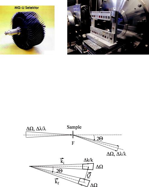
Fig. 5.1: Scheme of a small angle neutron scattering instrument. The neutrons pass from the left to the right. The incident beam is monochromated and collimated before it hits the sample. Nonscattered neutrons are absorbed by the beam stop in the center of the detector. The scattered neutron intensity is detected as a function of the scattering angle 2θ.

angle Ω. This solid angle is defined relatively to an ideally small sample and for large detector distances.

In practice, the classical small-angle neutron scattering apparatus including the source looks like this: In the reactor a nuclear chain reaction takes place. A uranium nucleus 235U captures a free neutron, and fission to smaller nuclei takes place. Additionally, 2.5 neutrons (on average) are released, which are slowed down to thermal energy by the moderator. One part of the neutrons keeps the chain reaction going, while the remaining part can be used for neutron experiments. The cold source is another moderator, which cools the neutrons to about 30K. Here, materials with light nuclei (deuterium at FRM 2) are used to facilitate the thermalization. The cold neutrons can easily be transported to the instruments by neutron guides. Rectangular glass tubes are used with a special mirror inside. The neutron velocity selector works mechanically (Fig. 5.1 shows scheme). A rotating cylinder with tilted lamellae allows only neutrons with a certain speed to pass (Fig. 5.2). The wavelengths distribution is ideally triangular with a relative half-width of ±5% or ±10%. The collimation determines the divergence of the beam. The entrance aperture and the sample aperture have a distance LC , and restrict the divergence of the beam. The sample is placed directly behind the sample aperture (Fig. 5.3). Many unscattered neutrons leave the sample and will be blocked by an absorber at the front of the detector. Only the scattered neutrons are detected by the detector at a distance LD. The sensitive detector detects about 93% of the scattered neutrons, but the huge primary beam cannot be handled, and, therefore, is absorbed by an absorber. In the instruments KWS-1 and KWS-2, the beam stop contains a small counter to measure the unscattered neutrons in parallel. The classic small-angle neutron scattering apparatus is also known as pinhole camera, because the entrance aperture is imaged to the detector by the sample aperture. The sample aperture may be opened further if focusing elements maintain (or improve) the quality of the image of the entrance aperture. By focusing elements the intensity of the experiment may be increased on the expense of needing large samples. Focusing elements can be either curved mirrors or neutron lenses made of MgF2. Both machines KWS-1 & KWS-2 have neutron lenses, but for this lab course they will not be used.

5.2.1 The scattering vector Q

In this section, the scattering vector Q is described with its experimental uncertainty. The scattering process is schematically shown in Fig. 5.4, in real space and momentum space. In real space the beam hits the sample with a distribution of velocities (magnitude and direction). The neutron speed is connected to the wavelength, whose distribution is depending on the velocity selector. The directional distribution is defined by the collimation. After the scattering process, the direction of the neutron is changed, but the principal inaccuracy remains the same. The scattering angle 2θ is the azimuth angle. The remaining polar angle is not discussed further here. For samples with no preferred direction, the scattering is isotropic and, thus, does not depend on the polar angle. In reciprocal space, the neutrons are defined by the wave vector k. The main direction of the incident beam is defined as the z-direction, and the modulus is determined by the wavelength, so |ki| = 2π/λ. Again, k is distributed due to the selector and the collimation inaccuracies. The wave vector of the (quasi) elastic scattering process has the same modulus, but differs in direction, namely by the angle 2θ. The difference between both wave vectors is given by the following value:

For isotropic scattering samples, the measured intensity depends only on the absolute value of the scattering vector Q = |Q|. For small angles, the common approximation of small angle (neutron) scattering is valid:

The typical Q-range of a small angle scattering instrument thus follows from the geometry. The detector distances LD vary in the range from 1m to 20m. The area detector is active between ØD = 2cm and 35cm from the center. The angle 2θ is approximated by the ratio ØD/LD and the wavelength λ varies between 4.5 and 20A˚ (typically 7A)˚ . For the instruments KWS-1 and KWS-2, a typical Q-range from 10−3 to 0.6A˚ −1 is obtained.

The Q-vector describes which length scales are observed, following the rule = 2π/Q. If a Bragg peak is observed, the lattice parameters can be taken directly from the position of the peak. If the scattering shows a sudden change at a certain Q-value, we obtain the length scale of the structural differences. There are characteristic scattering behaviors that can be described by so called scattering laws that are simple power laws Qα with different exponents α.

5.2.2 The Fourier transformation in the Born approximation

This section deals with the physical explanation for the appearance of the Fourier transformation in the Born approximation. In simple words, in a scattering experiment one observes the intensity as the quadrature of the Fourier amplitudes of the sample structure. This is considerably different from microscopy where a direct image of the sample structure is obtained. So the central question is: Where does the Fourier transformation come from?

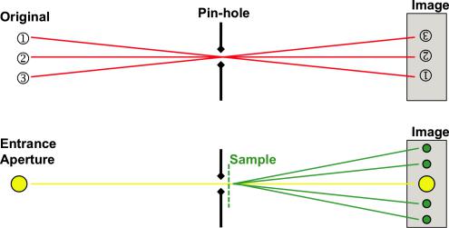
Fig. 5.5: The principle of a pin-hole camera transferred to the pin-hole SANS instrument. Top: The pin-hole camera depicts the original image (here consisting of three numbers). For simplicity, the three points are represented by three rays which meet in the pin-hole, and divide afterwards. On the screen, a real space image is obtained (upside down). Bottom: The pin-hole SANS instrument consists of an entrance aperture which is depicted on the detector through the pin-hole (same principle as above). The sample leads to scattering. The scattered beams are shown in green.

The classical SANS instruments are also called pin-hole instruments. Historically, pin-hole cameras were discovered as the first cameras. They allowed to picture real sceneries on blank screens – maybe at different size, but the image resembled the original picture. The components of this imaging process are depicted in Fig. 5.5. Let’s assume the following takes place with only one wavelength of light. The original image is then a monochromatic picture of the three numbers 1, 2 and 3. The corresponding rays meet in the pin-hole, and divide afterwards. On the screen, the picture is obtained as a real-space image, just appearing upside down. From experience we know that the screen may be placed at different distances resulting in different sizes of the image. The restriction of the three beams through the pin-hole holds for the right space behind the pin-hole. In front of the pin-hole the light propagates also in other directions

– it is just absorbed by the wall with the pin-hole.

So far, we would think that nothing special has happened during this process of reproduction. But what did happen to the light in the tiny pin-hole? We should assume that the size of the pinhole is considerably larger than the wavelength. Here, the different rays of the original image interfere and inside the pin-hole a wave field is formed. The momentum along the optical z-axis indicates the propagation direction, and is not very interesting (because is nearly constant for all considered rays). The momenta in the x-y-plane are much smaller and indicate a direction. They originate from the original picture and remain constant during the whole process. Before and after the pin-hole the rays are separated and the directions are connected to a real-space image. In the pin-hole itself the waves interfere and the wave field looks more complicated. The information about the original scenery is conserved through all the stages. That means that

also the wave field inside the pin-hole is directly connected to the original picture.

From quantum mechanics (and optics), we know that the vector of momentum is connected to a wave vector. This relation describes how the waves inside the pin-hole are connected to a spectrum of momenta. In classical quantum mechanics (for neutrons), a simple Fourier transformation describes how a wave field in real space (pin-hole state) is connected with a wave field in momentum space (separated beams). In principle, the interpretation is reversible. For electromagnetic fields (for x-rays), the concept has to be transferred to particles without mass. Overall, this experiment describes how the different states appear, and how they are related. The free propagation of a wave field inside a small volume (pin-hole) leads to a separation of different rays accordingly to their momentum.

Now we exchange the original image by a single source (see yellow spot in lower part of Fig. 5.5). This source is still depicted on the image plate (or detector). If we insert a sample at the position of the pin-hole, the wave field starts to interact with the sample. In a simplified way we can say that a small fraction of the wave field takes the real space structure of the sample while the major fraction passes the sample without interaction. This small fraction of the wave field resulting from the interaction propagates freely towards the image plate and generates a scattering pattern. As we have learned, the momenta present in the small fraction of the wave field give rise to the separation of single rays. So the real space image of the sample leads to a Fourier transformed image on the detector. This is the explanation, how the Fourier transformation appears in a scattering experiment – so this is a simplified motivation for the Born approximation. A similar result was found by Fraunhofer for the diffraction of light at small apertures. Here, the aperture is impressed to the wave field (at the pin-hole), and the far field is connected to the Fourier transformation of the aperture shape.

Later, we will see that the size of wave field packages at the pin-hole is given by the coherence volume. The scattering appears independently from such small sub-volumes and is a simple superposition.

5.2.3 Remarks on focusing instruments

We have described the resolution function of the pin-hole SANS instrument very well. This design comes to its limits if very large structures (of μm) need to be resolved. Usually focusing instruments take over because they provide higher intensities at higher resolutions.

Focusing instruments have the same motivation as photo cameras. When the pin-hole camera does not provide proper intensities any more, focusing elements – such as lenses – allow for opening the apertures. Then the resolution is good while the intensity increases to a multiple of its original value. For focusing SANS instruments this means that the sample sizes must be increased accordingly to the lens or mirror size.

There are two possible ways for focusing elements: Neutron lenses are often made of MgF2. Large arrays of lenses take an overall length of nearly one meter. This is due to the low refractive index of the material for neutrons. A disadvantage of the lenses is the dispersion relation which leads to strong chromatic aberrations. So it is hardly possible to focus the full wavelength band of classical neutron velocity selectors on the detector. Other ways like magnetic neutron lenses have to deal with similar problems.

Fig. 5.6: How a Fourier transformation is obtained with refractive lenses. The real space structure in the focus of the lens is transferred to differently directed beams. The focusing lens is concave since for neutrons the refractive index is smaller than 1.

The focusing mirror does not show chromatic aberration. So this focusing element provides the highest possible resolution at highest intensities. The small angle scattering instrument KWS- 3 is a unique instrument which uses this technique. The mirror technique was motivated by satellite mirrors. The roughness needs to stay below a few Angstr˚ om¨ over large areas.

Practically the entrance aperture may be closed to a few millimeters while the sample aperture takes a few square centimeters accordingly to the mirror size. This setup images the entrance aperture on the detector. So, the primary beam profile has sharp edges in comparison to the triangular shapes of the pin-hole camera. This narrower distribution of intensity means that the beam stop might be slightly smaller than for a similar pin-hole instrument and so the focusing instrument improves the intensity-resolution problem by a rough factor of two.

For a symmetric set-up (collimation and detector distance equal, i.e. LC = LD) the focusing optic is in the middle at the sample position. The focus f is half the collimation distance, i.e. f = 12 LC = 12 LD. Now the places where exact Fourier transforms are obtained (from the entrance aperture and from the sample structure) do not agree anymore. The sample is still considered as a small volume and from there the waves propagate freely to the detector, and the already known relation between sample structure and scattering image holds.

For focusing elements, the places of Fourier transformations differ (see Fig. 5.6). The original structure is placed in the focus, and the resulting distinctive rays are obtained at the other side of the lens in the far field. So for focusing SAS instruments, the places of appearing Fourier transformations for the entrance aperture and the sample structure differ.

The historical development of cameras can be seen in parallel. The first cameras were pin-hole cameras, but when lenses could be manufactured lens cameras replaced the old ones. The direct advantage was the better light yield being proportional to the lens size. Another effect appeared: The new camera had a depth of focus – so only certain objects were depicted sharply, which was welcomed in the art of photography. The focusing SAS instrument depicts only the entrance aperture, and the focusing is not a difficult task. The higher intensity or the better resolution are the welcomed properties of the focusing SAS instrument.

We therefore tend to subtract the incoherent scattering. It is well determined at large Q when the coherent scattering becomes small. The origin of the incoherent scattering is the spindependent scattering length. Especially for hydrogen 1H the neutron spin and the nuclear spin form a singlet or triplet state with different scattering lengths. The average scattering length of these two states contributes to the coherent scattering. The variance of the scattering length gives rise to the incoherent scattering. Here, each of the nuclei appears as an independent point scatterer which in reciprocal space means a Q-independent scattering signal. The dependence of the scattering on the neutron spin means that neutron spin polarization and analysis yields another method to determine the incoherent scattering independently from the coherent signal.

5.2.6 Resolution

The simple derivatives of equation 5.2 support a very simple view on the resolution of a small angle neutron scattering experiment. We obtain:

The uncertainty about the Q-vector is a sum about the uncertainty of the wavelength and the angular distribution. Both uncertainties result from the beam preparation, namely from the monochromatization and the collimation. The neutron velocity selector selects a wavelength band of either ±5% or ±10%. The collimation consists of an entrance aperture with a diameter dC and a sample aperture of a diameter dS. The distance between them is LC .

One property of eq. 5.7 is the changing importance of the two contributions at small and large Q. At small Q the wavelength spread is nearly negligible and the small terms Q and θ dominate the resolution. This also means that the width of the primary beam is exactly the width of the resolution function. More exactly, the primary beam profile describes the resolution function at small Q. Usually, the experimentalist is able to change the resolution at small Q. At large Q the resolution function is dominated by the wavelength uncertainty. So the experimentalist wants to reduce it – if possible – for certain applications. This contribution is also an important issue for time-of-flight SANS instruments at spallation sources. The wavelength uncertainty is determined by the pulse length of the source and cannot be reduced without intensity loss.

A more practical view on the resolution function includes the geometrical contributions explicitely [3]. One obtains:

Now the wavelength spread is described by λ being the full width at the half maximum. The geometrical terms have contributions from the aperture sizes dC and dS and the spatial detector

resolution dD. The collimation length LC and detector distance LD are usually identical such that all geometric resolution contributions are evenly large (dC = 2dS then). This ideal setup maximizes the intensity with respect to a desired resolution.

The resolution function profile is another topic of the correction calculations. A simple approach assumes Gaussian profiles for all contributions, and finally the overall relations read:

The theoretical macroscopic cross section is often described by a model function which is fitted to the experimental data. In this case the computer program only does a convolution of the model function with the resolution function R(ΔQ). Alternatively, there are methods to deconvolute the experimental data without modeling the scattering at first hand.

The here described resolution function is given as a Gaussian. This is true for relatively narrow distributions. The reason for using a Gaussian function although the original distributions of λ and θ are often triangular is: The central limit theorem can be applied to this problem because we have seen from eq. 5.8 that there are four contributions to the resolution function, and the radial averaging itself also smears the exact resolution function further out. Thus, the initial more detailed properties of the individual distributions do not matter anymore. Equations 5.9 and 5.10 are a good approximation for many practical cases.

We now want to describe the connection between the resolution function and the coherence of the neutron beam at the sample position. From optics we know about the transverse coherence length:

It can be compared well with the geometric resolution contribution that arises from the entrance aperture only. Small differences in the prefactors we can safely neglect. For the longitudinal coherence length we obtain:

This coherence length can be well compared to the wavevector uncertainty of the incoming beam. If we look back on Figure 5.4 we see that the coherence volume exactly describes the uncertainty of the incoming wave vector. The two contributions are perpendicular which supports the vectorial (independent) addition of the contributions in eq. 5.8 for instance. The coherence volume describes the size of the independent wave packages which allow for wave-like properties such as the scattering process. So the coherence volume describes the maximum size

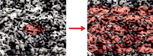
Fig. 5.7: The coherence volume is usually much smaller than the sample volume (left). So the overall scattering appears as an incoherent superposition of the scattering from many coherence volumes (right).

of structure that is observable by SANS. If larger structures need to be detected the resolution must be increased.

The understanding how the small coherence volume covers the whole sample volume is given in the following (see also Fig. 5.7). Usually the coherence volume is rather small and is many times smaller than the irradiated sample volume. So many independent coherence volumes cover the whole sample. Then, the overall scattering intensity occurs as an independent sum from the scattering intensities of all coherence volumes. This is called incoherent superposition.

5.3The theory of the macroscopic cross section

We have seen that the SANS instrument aims at the macroscopic cross section which is a function of the scattering vector Q. In many examples of isotropic samples and orientationally averaged samples (powder samples) the macroscopic cross section depends on the modulus |Q| ≡ Q only. This measured function has to be connected to important structural parameters of the sample. For this purpose model functions are developed. The shape of the model function in comparison with the measurement already allows to distinguish the validity of the model. After extracting a few parameters with this method, deeper theories – like thermodynamics – allow to get deeper insight about the behavior of the sample. Usually, other parameters – like concentration, temperature, electric and magnetic fields, ... – are varied experimentally to verify the underlying concepts at hand. The purpose of this section is to give some ideas about model functions.

When the Born approximation was developed several facts and assumptions came along. The scattering amplitudes of the outgoing waves are derived as perturbations of the incoming plane wave. The matrix elements of the interaction potential with these two wave fields as vectors describe the desired amplitudes. The interaction potential can be simplified for neutrons and the nuclei of the sample by the Fermi pseudo potential. This expresses the smallness of the nuclei ( 1fm) in comparison to the neutron wavelength ( A)˚ . For the macroscopic cross section we