

Schluesseltech_39 (1)
.pdf5.14 |
H. Frielinghaus |
|
|
immediately obtain a sum over all nuclei:
dΩ(Q) = |
V |
|
j |
2 |
(5.13) |
||
|
bj exp(iQ · rj ) |
||||||
dΣ |
1 |
|
|
|
|||
|
|
|
|
|
|
||
|
|
|
|
|
|
|
|
|
|
|
|
|
|
|
|
This expression is normalized to the sample volume V because the second factor usually is proportional to the sample size. This simply means: The more sample we put in the beam the more intensity we obtain. The second factor is the square of the amplitude because we measure intensities. While for electromagnetic fields at low frequencies one can distinguish amplitudes and phases (without relying on the intensity) the neutrons are quantum mechanical particles where experimentally such details are hardly accessible. For light (and neutrons) for instance holographic methods still remain. The single amplitude is a sum over each nucleus j with its typical scattering length bj and a phase described by the exponential. The square of the scattering length b2j describes a probability of a scattering event taking place for an isolated nucleus. The phase arises between different elementary scattering events of the nuclei for the large distances of the detector. In principle, the scattering length can be negative (for hydrogen for instance) which indicates an attractive interaction with a phase π. Complex scattering lengths indicate absorption. The quadrature of the amplitude can be reorganized:
dΣ |
1 |
|
|
|
||
|
|
(Q) = |
|
|
bj bk exp iQ(rj − rk) |
(5.14) |
dΩ |
V |
j,k |
||||
|
|
|
|
|
|
|
Here we find then self-terms with identical indices j and k without any phase and cross terms with phases arising from distances between different nuclei. Here it becomes obvious that only relative positions of the nuclei matter which is a result of the quadrature. The overall phase of the sample does not matter because of the modulus in eq. 5.13. We will use this expression for the polymer scattering.
Apart from this detailed expression a simplified view is allowed for small angle scattering experiments. Firstly, we know that the wavelength is typically 7A˚ which is much larger than the atom-atom distance of ca. 1.5A˚ . Secondly, the SANS experiment aims at structures at the nanoscale. So the scattering vector aims at much larger distances compared to the atomistic distances (i.e. 2πQ−1 1A)˚ . This allows for exchanging sums by integrals as follows:
j |
bj · · · |
−→ |
|
d3r ρ(r) · · · |
(5.15) |
|
|
|
V |
|
|
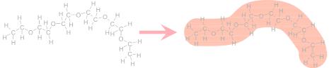
Such methods are already known for classical mechanics, but reappear all over physics. The meaning is explained by the sketch of Figure 5.8. The polymer polyethylene oxide (PEO) contains many different nuclei of different species (hydrogen, carbon and oxide). However, the SANS method does not distinguish the exact places of the nuclei. The polymer appears rather like a homogenous worm. Inside, the worm has a constant scattering length density which reads:
|
1 |
|
{ |
|
ρmol = Vmol |
|
|
||
j |
bj |
(5.16) |
||
|
|
mol} |
|
|
Nanostructures investigated by SANS |
5.15 |
|
|
Fig. 5.8: The concept of the scattering length density. On the left the atomic structure of a polyethylene oxide polymer (PEO) is depicted. For small angle scattering the wavelength is much larger than the atomic distance. So for SANS the polymer appears like a worm with a constant scattering length density inside.
So, for each molecule we consider all nuclei and normalize by the overall molecule volume. Of course different materials have different scattering length densities ρ. The initial equation 5.13 reads then:
2
dΩ(Q) = |
V |
d3r ρ(r) exp(iQr) |
|
|
|
|
|
|
(5.17) |
||||
dΣ |
1 |
V |
|
|
|
|
|
|
|
|
|
|
|
|
|
|
|
|
|
|
|
|
|
|
|
||
|
1 |
|
|
|
2 |
|
|
1 |
|
|
|
2 |
|
|
|
|
|
|
|
|
|
|
|
|
|||
= |
|
|
[ρ(r)] |
|
|
|
= |
|
|
|
ρ(Q) |
|
(5.18) |
V |
|
V |
|||||||||||
|
F |
|
|
|
|
|
|
||||||
|
|
|
|
|
|
|
|
|
|
|
|
|
|
|
|
|
|
|
|
|
|
|
|
|
|
|
|
The single amplitude is now interpreted as a Fourier transformation of the scattering length density ρ(r) which we simply indicate by ρ(Q). The amplitude simply is defined by:
ρ(Q) = d3r ρ(r) exp(iQr) (5.19)
V
Again, equation 5.17 loses the phase information due to the modulus. While we focused on the scattering experiment so far, another view on this function will provide us with further insight. We define the correlation Γ as follows:
Γ(Q) = V |
ρ(Q) |
= |
V ρ (Q)ρ(Q) = |
V ρ(−Q)ρ(Q) |
(5.20) |
|||||
1 |
|
2 |
1 |
|
1 |
|
|
|||
|
|
|
|
|
|
|
|
|
|
|
|
|
|
|
|
|
|
|
|
|
|
The modulus is usually calculated via the complex conjugate ρ (Q) which in turn can be obtained by changing the sign of the argument Q. Now the correlation function is a simple product of two Fourier transformed functions. They can be interpreted on the basis of a convolution in real space:
Γ(r) = V ρ(r) ρ(r) = |
V |
V |
d3r ρ(r + r ) · ρ(r ) |
(5.21) |
|
1 |
|
1 |
|
|
|
The underlying correlation function Γ(r) arises from the convolution of the real space scattering length density with itself. The mathematical proof is carried out in Appendix A. For imagining
5.16 |
H. Frielinghaus |
|
|
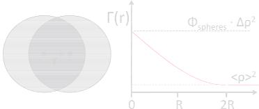
Fig. 5.9: On the left the meaning of the convolution is depicted. Two identical shapes are displaced by a vector r. The convolution volume is the common volume (dark grey). This consideration leads for three-dimensional spheres to the linear correlation function Γ(r) shown on the right.
the convolution assume you have two foils with the same pattern printed on. The vector r describes the relative displacement of the two foils. Then you calculate the product of the two patterns and integrate over V . For patterns of limited size it becomes clear that the function turns to ‘zero’ at a finite distance r. For simple compact patterns the function monotonically decays. The example of spheres is depicted in Fig. 5.9. In the left the meaning of the convolution is indicated. The darkest area in the center is the considered volume of the convolution for the vector r. In three dimensions this consideration leads to the correlation function (see also Appendix A and references [4, 5]):
spheres · |
|
· |
0 |
− |
|
| | |
| | |
|
for |r| > 2R |
|
|
Γ(r) = φ |
ρ2 |
|
1 |
|
23 |
r /(2R) + 21 |
r |
3/(2R)3 |
for |r| ≤ 2R |
+ ρ |
2 (5.22) |
The concentration φspheres accounts for many independent, but diluted spheres. The value ρ is the scattering length density difference between the sphere and the surrounding matrix (i.e. solvent). The constant ρ 2 is the average scattering length density of the overall volume. Apart from these simple rationalizations we can formally calculate the limits for small and large distances r:
Γ(r → 0) = ρ2 |
|
|
Γ(r → ∞) = ρ 2 |
(5.23) |
|
At this stage the reasons for the limits are |
based on mathematics. The brackets |
· · · |
indi- |
||
|
2 |
|
|
||
cate an averaging of a locally defined function ρ |
|
(r), ρ(r) over the whole volume. For small |
|||
distances the averaging over squares of the scattering length density usually leads to higher values compared to the average being squared afterwards. So the correlation function often is a monotonically decaying function. A very simple realization is given by:
Γ(r) = |
|
ρ − |
ρ |
|
2 exp |
−|r|/ξ |
+ ρ 2 |
(5.24) |
|
|
|
|
|
|
|
|
Nanostructures investigated by SANS |
5.17 |
|
|
The shape of the decay is usually described by an exponential decay and can be motivated further in detail [1]. The first addend is proportional to the fluctuations of the scattering length density. This finding already indicates that scattering experiments are sensitive to fluctuations. The correlation length ξ indicates over which distance the correlations are lost. The current picture does not allow for a complete decay (in comparison to the single sphere which finds Γ(r) = 0 for r > 2R). This means that the current discussion treats scattering length density fluctuations which fill the full 3-dimensional space. The Fourier transformation of eq. 5.24 leads to the following expression:
Γ(Q) |
|
ρ − ρ |
|
2 |
1 +ξξ32Q2 |
(5.25) |
|
|
|
|
|
|
|
|
|
The scattering intensity in this case is proportional to the scattering length density fluctuations, to the coherence volume ξ3 and the Q-dependent Lorentz peak. The latter has to be interpreted as a kind of expansion. So different details of the decaying correlation function (eq. 5.24) might lead to differently decaying scattering functions. The current Lorentz function is typical for Ornstein-Zernicke correlation functions. Further discussions of the correlation function are given in Appendix A.
For the fluctuations of the scattering length density we would like to consider a two phase system, i.e. the whole space is taken by either component 1 or 2. The concentration of phase 1 is φ1, and the scattering length density is ρ1 (correspondingly ρ2 is defined). For the average scattering lenght density we clearly obtain ρ = φ1ρ1 + (1 − φ1)ρ2. For the scattering length density fluctuations we obtain similarly (ρ − ρ )2 = φ1(1 − φ1)(ρ1 − ρ2)2. The latter result describes the concentration fluctuations of the two phase system and the scattering length density contrast. For the following considerations the contrast will reappear in many examples.
5.3.1 Spherical colloidal particles
In this section we will derive the scattering of diluted spherical particles in a solvent. These particles are often called colloids, and can be of inorganic material while the solvent is either water or organic solvent. Later in the manuscript interactions will be taken into account.
One important property of Fourier transformations is that constant contributions will lead to sharp delta peaks at Q = 0. This contribution is not observable in the practical scattering experiment. The theoretically sharp delta peak might have a finite width which is connected to the overall sample size, but centimeter dimensions are much higher compared to the largest sizes observed by the scattering experiment ( μm). So formally we can elevate the scattering density level by any number −ρref :
ρ(r) −→ ρ(r) − ρref leads to ρ(Q) −→ ρ(Q) − 2πρref δ(Q) |
(5.26) |
The resulting delta peaks can simply be neglected. For a spherical particle we then arrive at the simple scattering length density profile:
ρ |
single |
(r) = |
|
ρ |
for |r| ≤ R |
(5.27) |
|
|
0 |
for |r| > R |
|

5.18 |
H. Frielinghaus |
|
|
Inside the sphere the value is constant because we assume homogenous particles. The reference scattering length density is given by the solvent. This function will then be Fourier transformed accordingly:
ρsingle(Q) = |
2πdφ |
π dϑ sin ϑ |
R dr r2 |
ρ exp i|Q| · |r| cos(ϑ) |
(5.28) |
|
0 |
0 |
0 |
|
|
= |
2π |
R |
dr r2 |
iQr exp |
|
iQrX |
||
ρ |
|
|||||||
|
|
|
|
1 |
|
|
|
|
|
|
0 |
|
|
|
|
||
= |
4π |
R |
dr r2 |
|
Qr |
|
|
|
ρ |
|
|
|
|||||
|
|
|
|
sin(Qr) |
|
|
||
X=+1
(5.29)
X=−1
(5.30)
|
0 |
|
|
|
|
||
= ρ |
4π |
R3 |
|
3 |
sin(QR) − QR cos(QR) |
(5.31) |
|
3 |
|||||||
|
|
|
(QR)3 |
|
|||
In the first line 5.28 we introduce spherical coordinates with the vector Q determining the z- axis for the real space. The vector product Qr then leads to the cosine term. In line 5.29 the azimutal integral is simply 2π, and the variable X = cos ϑ is introduced. Finally, in line 5.30 the kernel integral for spherically symmetric scattering length density distributions is obtained. For homogenous spheres we obtain the final result of eq. 5.31. Putting this result together for the macroscopic cross section (eq. 5.18) we obtain:
dΩ(Q) = |
V |
|
· ρsingle(Q) |
= (Δρ)2 φspheres Vsphere F (Q) |
(5.32) |
|||
dΣ |
N |
|
|
2 |
|
|
|
|
|
|
|
|
|
|
2 |
|
|
|
|
|
sin( |
(QR)3 |
|
|
|
|
F (Q) = |
|
3 |
QR) − QR cos(QR) |
|
(5.33) |
|||
|
|
|
||||||
|
|
|
|
|||||
We considered N independent spheres in our volume V , and thus obtained the concentration of spheres φspheres. Furthermore, we defined the form factor F (Q), which describes the Q- dependent term for independent spheres (or the considered shapes in general). The function is shown in Figure 5.10. The first zero of the form factor is found at Q = 4.493/R. This relation again makes clear why the reciprocal space (Q-space) is called reciprocal. We know the limit for small scattering angles is F (Q → 0) = 1 − 15 Q2R2. So the form factor is normalized to 1, and the initial dependence on Q2 indicates the size of the sphere. For large scattering angles the form factor is oscillating. Usually the instrument cannot resolve the quickest oscillations and an average intensity is observed. The asymptotic behavior would read F (Q→∞) = 92 (QR)−4. The obtained power law Q−4 is called Porod law and holds for any kind of bodies with sharp interfaces. So, sharp interfaces are interpreted as fractals with d = 2 dimensions, and the corresponding exponent is 6 − d. The general appearance of the Porod formula reads then:
dΣ |
(Q) = P · Q−4 |
(5.34) |
dΩ |
Nanostructures investigated by SANS |
5.19 |
|
|
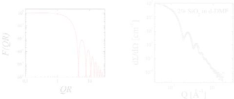
Fig. 5.10: The form factor of a homogenous sphere in a double logarithmic plot.
Fig. 5.11: Experimental scattering curve of spherical SiO2 colloids in the deuterated solvent DMF [6]. The resolution function (eq. 5.9) is included in the fit (red line).
The amplitude of the Porod scattering P tells about the surface per volume and reads P = 2π(Δρ)2Stot/Vtot. Apart from the contrast, it measures the total surface Stot per total volume Vtot. For our shperes, the Porod constant becomes P = 2π(Δρ)24πR2/(4πR3/(3φ)) = 6πφ1(Δρ)2/R. The surface to volume ratio is smaller the larger the individual radius R is. The remaining scaling with the concentration φ1 and the contrast (Δρ)2 arises still from the prefactor which we discussed in context with eq. 5.32.
When comparing the theoretical description of the spherical form factor with measurements one finds a good agreement (Fig. 5.11). Many fringes are seen, but after the third or fourth peak the function does not indicate any oscillation any more. Furthermore, the sharp minima are washed out. All of this is a consequence of the resolution function (eq. 5.9) which has been taken into account for the fitted curve. For many other examples one also needs to take the polydispersity into account. The synthesis of colloids usually produces a whole distribution of different radii. In our example the polydispersity is very low which is the desired case. Polydispersity acts in a similar way compared to the resolution function. The sharp minima are washed out. While the resolution appears as a distribution of different Q-values measured at a certain point the polydispersity integrates over several radii.
Another general scattering law for isolated (dilute) colloids is found for small scattering angles. The general appearance of the Guinier scattering law is:
|
dΩ |
(Q→0) = dΩ(0) · exp |
−3Q2Rg2 |
|
|
(5.35) |
|||
|
dΣ |
dΣ |
1 |
|
|
|
|
|
|
|
|
|
|
||||||
When comparing the scattering law of a sphere and the Guinier formula we obtain Rg = |
|
3 R. |
|||||||
|
|
|
|
|
|
|
5 |
|
|
The radius of gyration Rg can be interpreted as a momentum of inertia normalized to |
the total |
||||||||
|
|
|
|||||||
mass and specifies the typical size of the colloid of any shape. The Guinier formula can be seen
5.20 |
H. Frielinghaus |
|
|
as an expansion at small scattering angles of the logarithm of the macroscopic cross section truncated after the Q2 term. Further details are discussed in Appendix B.
Another general appearance for independent colloids shall be discussed now using equation 5.32. The macroscopic cross section is determined by several important factors: The contrast between the colloid and the solvent given by ρ2, the concentration of the colloids, the volume of a single colloid, and the form factor. Especially for small Q the latter factor turns to 1, and the first three factors dominate. When knowing two factors from chemical considerations, the third factor can be determined experimentally using small angle neutron scattering.
When comparing this expression for isolated colloids with the Ornstein-Zernicke result we see in parallel: The contrast stays for both kinds of interpretations. The particle volume corresponds to the correlation volume (i.e. V ξ3). The concentration of the correlation volumes comes close to 1 (i.e. φ 1). Finally, F is a measure for the correlations inside the correlation volume. So, for independent colloids the correlation volume must fully cover the single particle but two neighbored particles are found in distinct correlation volumes. Finally, the overall experimental correlation length is limited by the sample and the radiation coherence. So, for the transversal correlation length one would obtain ξe−2,transv = ξ−2 + −coh2 ,transv.
5.3.2 Contrast variation
For neutron scattering the method contrast variation opens a wide field of possible experiments. For soft matter research the most important labelling approach is the exchange of hydrogen 1H by deuterium 2H. Since in a single experiment the phase information is lost completely the contrast variation experiment retrieves this information partially. Relative positions of two components are obtained by this method.
The scattering length density of the overall sample is now understood to originate from each component individually. So the specific ρj(r) takes the value of the scattering length density of component j when the location points to component j and is zero otherwise. We would then obtain the following:
ρ(Q) = |
d3r |
n |
ρj (r) exp(iQr) |
(5.36) |
|
|
|
|
|
Vj=1
n specifies the number of components. The assumption of incompressibility means that on every place there is one component present, and so all individual functions ρj (r) fill the full space. Furthermore, we would like to define component 1 being the reference component, i.e. ρref = ρ1 (see eq. 5.26). This means that on each place we have a ρj(r) function similar to eq. 5.22. Then, we arrive at:
n
ρ(Q) = |
ρj1(Q) |
(5.37) |
|
j=2 |
|
The macroscopic cross section is a quadrature of the scattering length density ρ(Q), and so we arrive at:
Nanostructures investigated by SANS |
5.21 |
|
|
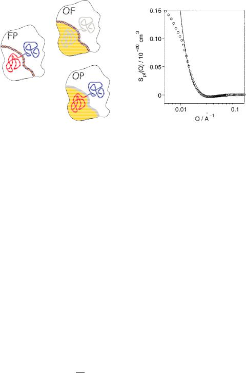
Fig. 5.12: Scheme of scattering functions for the cross terms within the microemulsion. There are the film-polymer scattering SFP, the oil-film scattering SOF, and the oil-polymer scattering SOP. The real space correlation function means a convolution of two structures.
Fig. 5.13: A measurement of the filmpolymer scattering for a bicontinuous microemulsion with a symmetric amphiphilic polymer. The solid line is described by a polymer anchored in the film. The two blocks are mushroom-like in the domains. At low Q the overall domain structure (or size) limits the idealized model picture.
dΣ |
1 |
|
n |
|
|
|
|
|||
|
|
ρj1(Q) · ρk1(Q) |
|
|||||||
|
|
(Q) = |
|
|
· |
(5.38) |
||||
|
dΩ |
|
V |
|
||||||
|
|
|
|
|
j,k=2 |
|
|
|
|
|
|
|
|
|
n |
|
|
|
|
|
|
= |
|
(Δρj1 |
|
ρk1) · Sjk(Q) |
|
(5.39) |
||||
|
|
|
j,k=2 |
|
|
|
|
|
||
|
|
|
|
n |
|
|
2 |
≤ |
|
|
|
|
|
|
|
|
(Δρj1 ρk1) · Sjk(Q) (5.40) |
||||
= |
|
|
(Δρj1)2 |
· Sjj(Q) + 2 |
|
|||||
|
|
|
|
j=2 |
|
|
|
<j<k |
n |
|
In line 5.39 the scattering function Sjk(Q) is defined. By this the contrasts are separated from the Q-dependent scattering functions. Finally, in line 5.40 the diagonal and off-diagonal terms are collected. There are n−1 diagonal terms, and 12 (n−1)(n−2) off-diagonal terms. Formally, these 12 n(n − 1) considerably different terms are rearranged (the combinations {j, k} are now simply numbered by j), and a number of s different measurements with different contrasts are considered.
dΩ(Q) s |
= |
j |
(Δρ · ρ)sj · Sj (Q) |
(5.41) |
|
dΣ |
|
|
|
|
|
5.22 |
H. Frielinghaus |
|
|
In order to reduce the noise of the result, the number of measurements s exceeds the number of independent scattering functions considerably. The system then becomes over-determined when solving for the scattering functions. Formally one can nonetheless write:
Sj (Q) = |
s |
(Δρ · |
ρ)sj−1 · dΩ(Q) s |
(5.42) |
|
|
|
|
dΣ |
|
|
The formal inverse matrix (Δρ· ρ)−sj1 is obtained by the singular value decomposition method. It describes the closest solution of the experiments in context of the finally determined scattering functions.
An example case is discussed for a bicontinuous microemulsion with an amphiphilic polymer [7]. The microemulsion consists of oil and water domains which have a sponge structure. So the water domains host the oil and vice versa. The surfactant film covers the surface between the oil and water domains. The symmetric amphiphilic polymer position and function was not clear beforehand. From phase diagram measurements it was observed that the polymer increases the efficiency of the surfactant dramatically. Much less surfactant is needed to solubilize equal amounts of oil and water. Fig. 5.12 discusses the meaning of the cross terms of the scattering functions. Especially the film-polymer scattering is highly interesting to reveal the polymer role inside the microemulsion (see Fig. 5.13). By the modeling it was clearly observed that the amphiphilic polymer is anchored in the membrane and the two blocks describe a mushroom inside the oil and water domains. So basically, the polymer is a macro-surfactant. The effect of the polymer on thermodynamics and the microscopic picture is discussed in chapter 5.3.5.
5.3.3 Scattering of a polymer
In this section we derive the scattering of a single (isolated) polymer coil. This model is the basis for many more complicated models of polymers in solution, polymeric micelles, polymer melts, diblock and multiblock copolymers and so on. So the understanding of these concepts is rather important for scattering experiments on any kind of polymer systems.
This example starts apart from many other calculations from point-like monomers (see eq. 5.14). These monomers are found along a random walk with an average step width of K . We try to argue for non-ideal chain segments, but finally will arrive at an expression for rather ideal polymers. For the scattering function we obtain (definition of S(Q) in eq. 5.39-5.41):
N
S(Q)
1
N
j,k=0
N
1
N
j,k=0
N
1
N
exp (iQ · (Rj − Rk)) |
(5.43) |
|
exp − |
21 (Q · (Rj − Rk))2 |
(5.44) |
exp − |
61 Q2 · (Rj − Rk)2 |
(5.45) |
j,k=0

Nanostructures investigated by SANS |
5.23 |
|
|
At this stage we use statistical arguments (i.e. statistical physics). The first rearrangement of terms (line 5.44) moves the ensemble average of the monomer positions (and distances Rjk) from the outside of the exponential to the inside. This is an elementary step which is true for polymers. The underlying idea is that the distance Rjk arises from a sum of |j − k| bond vectors which all have the same statistics. So each sub-chain with the indices jk is only distinguished by its number of bond vectors inside. The single bond vector bj has a statistical
average of b |
j |
= |
0 because there is no preferred orientation. The next higher moment is the |
||||
|
2 |
2 |
|
with an |
|||
second moment |
bj |
= K . This describes that each bond vector does |
2a finite step |
||||
2 |
|||||||
average length of K . For the sub-chain we then find an average size Rjk = |j − k| K . The reason is that in the quadrature of the sub-chain only the diagonal terms contribute because two distinct bond vectors show no (or weak) correlations.
Back to the ensemble average: The original exponential can be seen as a Taylor expansion with all powers of the argument iQ Rjk. The odd powers do not contribute with similar arguments than for the single bond vector bj = 0. Thus, the quadratic term is the leading term. The reason why the higher order terms can be arranged that they finally fit to the exponential expression given in line 5.44 is the weak correlations of two distinct bond vectors. The next line 5.45 basically expresses the orientational average of the sub-chain vector Rjk with respect to the Q-vector in three dimensions.
This derivation can be even simpler understood on the basis of a Gaussian chain. Then every bond vector follows a Gaussian distribution (with a center of zero bond length). Then the
ensemble average has the concrete meaning · · · = |
· · · exp |
− 23 |
Rjk2 /(|j −k| K2 ) d3 Rjk. |
|
This distribution immediately explains the |
rearrangement of line 5.44. The principal argument |
|||
|
|
|
|
|
is the central limit theorem: When embracing several segments as an effective segment any kind of distribution converges to yield a Gaussian distribution. This idea came from Kuhn who formed the term Kuhn segment. While elementary bonds still may have correlations at the stage of the Kuhn segment all correlations are lost, and the chain really behaves ideal. This is the reason why the Kuhn segment length K was already used in the above equations.
In the following we now use the average length of sub-chains (be it Kuhn segments or not), and replace the sums by integrals which is a good approximation for long chains with a large number of segments N.
S(Q) |
|
|
|
N |
N |
dk exp −61 Q2 · |j − k| · K2 |
(5.46) |
|
N |
dj |
|||||
|
|
1 |
|
|
|
|
|
|
|
0 |
0 |
|
|
||
|
= |
N · fD(Q2Rg2) |
(5.47) |
||||
fD(x) |
= |
|
2 |
(exp(−x) − 1 + x) |
(5.48) |
||
|
x2 |
||||||
In this integral one has to consider the symmetry of the modulus. The result is basically the Debye function which describes the polymer scattering well from length scales of the overall coil down to length scales where the polymer becomes locally rigid (see Fig. 5.14). The covalent
bonds of a carbon chain effectively contribute to a certain rigidity which will not be treated here.
The radius of gyration describes the overall dimension of the chain and is Rg = N/6 K . The limits of the polymer scattering are found to be: