

Schluesseltech_39 (1)
.pdf9.10 |
E. Kentzinger |
Fig. 9.6: Roughness of a real interface, characterized by the parametrization pendency of the refractive index on z.
2 |
− |
−2 |
erf √2σj |
|
|||
n(z) = |
nj + nj+1 |
|
nj |
nj+1 |
|
z − zj |
|
|
|
|
|
|
|
|
|
with the “Error” function: |
|
|
|
|
|
|
|
z(x, y) and de-
(9.25)
erf(z) = √π 0 |
e−t |
dt. |
(9.26) |
|
2 |
|
z |
|
|
|
2 |
|
|
|
The reflectivity from such a rough interface is obtained from the average of the reflectivities from a sequence of layers that describe the profile of refraction index. This average is performed in detail in Ref. [6]. As a result one obtains that the Fresnel coefficient for an ideally flat interface has to be modified by an exponential damping factor in the following way:
Rrough = Rflat · exp −4σj2kzjkzj+1 . |
(9.27) |
In this equation, σj is the root mean squared deviation from the nominal position of the flat interface.
The effects of interfacial roughness on the neutron reflectivity from a Si substrate and from a Ni layer on Si substrate have been simulated in Fig. 9.7. On the left side of Fig. 9.7 one can observe that the effect of roughness is to decrease the reflectivity at large wave vector transfers. The effect of roughness will be seen, if the value of the scattering wave vector gets bigger than 1/σ. Therefore, if one wants to determine very small roughness amplitudes, one has to measure the reflectivity till very large reflection angles and over a large dynamical range.
The right side of Fig. 9.7 shows the effect of the roughness of a single layer. The simulations have been performed for ideally flat interfaces, for a rough surface of the layer, for a rough interface between layer and substrate and for the case where both interfaces are rough. One can

Neutron reflectometry |
9.11 |
see that the four cases can be well differentiated. When only one of the two interfaces is rough, the interference pattern due to the reflection on the top and bottom interfaces is suppressed at large wave vectors. If both interfaces are rough, a faster decrease of the averaged reflectivity takes place.
|
1 |
|
no roughness |
|
1 |
|
no roughness |
|
|||||
|
|
|
|
σ = 5 |
Å |
|
|
|
|
σNi |
= 15 |
Å |
|
|
0.01 |
|
|
σ = 20 |
Å |
|
0.01 |
|
|
σSi |
= 15 |
Å |
|
Reflectivity |
|
|
|
|
|
|
σNi =σSi |
= 15 |
Å |
|
|||
0.0001 |
|
|
|
|
|
0.0001 |
|
|
|
|
|
|
|
|
|
|
|
|
|
|
|
|
|
|
|
|
|
|
1e−06 |
|
|
|
|
|
1e−06 |
|
|
|
|
|
|
|
0 |
0.04 |
0.08 |
0.12 |
0.16 |
0.2 |
0 |
0.04 |
0.08 |
0.12 |
0.16 |
0.2 |
|
|
|
Q = 4π/λsin(θ) [Å −1] |
|
|
Q = 4π/λsin(θ) [Å −1] |
|
|||||||
Fig. 9.7: Left: Neutron reflectivity at the interface between vacuum and Si. Right: Neutron reflectivity from a 400 A˚ thick Ni layer on Si substrate. Effect of interfacial roughness.
Finally, one should point out that a specular reflectivity measurement can only describe the profile of scattering length density normal to the interface. This means that a reflectivity measurement can not differentiate between interfacial roughness and interdiffusion, as interdiffusion will induce the same profile of refraction index as in Fig. 9.6. But what happens to the intensity loss described by the exponential factor of Eq. (9.27)? In the case of a diffuse interface, this intensity goes into the transmitted beam because there is no potential gradient in a direction different than the one normal to the interface. On the other hand, in the case of a rough interface, the intensity loss comes from scattering by lateral fluctuations of the potential, leading to intensities that can be observed in directions other than the specular direction: this is off-specular diffuse scattering. A statistical function like the height-height pair correlation function can be determined from the measurement of off-specular scattering [5].
9.3 Neutron reflectivity measurement and data analysis
The principal components of a reflectivity experiment are (i) a radiation source, (ii) a wavelength selector (monochromator, choppers), (iii) a collimation system, (iv) the sample and (v) a detection system.
The aim of a neutron specular reflectivity experiment is to measure the reflectivity as a function of the scattering wave vector Q perpendicular to the sample surface:
Q = |
4π |
sin θ |
(9.28) |
|
|||
|
λ |
|
|
9.12 |
E. Kentzinger |
The measurement can be done by changing either the angle of incidence θ on the sample or the wavelength λ, or both.
9.3.1 Monochromatic instruments
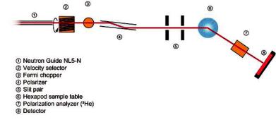
At a nuclear reactor source, the measurements are usually performed at a fixed value of λ, using θ-2θ scans (2θ being the detector angle). The wavelength selection can be obtained by Bragg scattering on a monochromator crystal or by using a velocity selector. Fig. 9.8 describes such an instrument. This is the MARIA reflectometer of the JCNS located at the FRM-II source in Garching [7]. The neutrons are brought from the cold source to the instrument using a supermirror coated guide (see lecture 2 of this book). A certain wavelength with a spread of 10 % is chosen by adjusting the rotation speed of a velocity selector. The wavelength spread can be reduced by using a Fermi chopper and time-of-flight detection. The neutron beam is then collimated by a pair of slits in order to define the angle of incidence of the neutrons relative to the sample surface with a certain precision. The neutrons are then detected on a two dimensional position sensitive detector. Such a detector allows to record at the same time not only the specular reflectivity signal but also the signals of off-specular scattering and grazing incidence small angle scattering. The projection of the spin of the neutron on a quantization axis can be selected before interaction with the sample by using a polarizer and after interaction with the sample by using a polarization analyzer, allowing to retrieve information about the norm and angle of the layer magnetizations in a magnetic sample (see lecture 10). The polarizer uses magnetic supermirrors and the analyzer uses a nuclear polarized 3He gas to select the spin projection.
Fig. 9.8: A monochromatic instrument: MARIA of the JCNS at FRM-II [7].
9.3.2 Time-of-flight instruments
At a spallation source, the measurements are performed at fixed values of θ and as a function of λ. This is the time-of-flight technique, that consists in sending a pulsed white beam on the sample. Since the speed of the neutron varies as the inverse of the wavelength, the latter is directly related to the time taken by the neutron to travel from the pulsed source to the detector (over the distance L) by:
Neutron reflectometry |
|
|
9.13 |
|
λ = |
h |
t. |
(9.29) |
|
mL |
||||
|
|
|
For a reflectivity measurement, the angle is fixed and the reflectivity curve is obtained by measuring the reflectivity signal for each wavelength of the available spectrum, each wavelength corresponding to a different scattering wave-vector magnitude. Sometimes it is necessary to use several angles of incidence because the Q range is not large enough.
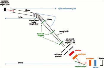
An example of time-of-flight reflectometer is presented in Fig. 9.9. This is the magnetism reflectometer of the Spallation Neutron Source (SNS) in Oak Ridge, USA [8]. Neutrons coming from the moderator are first deflected by 2.5o using a channel beam bender, composed of a stack of supermirrors, in order to achieve enough separation with the neighbour instrument (a liquid reflectometer) and in order to deliver to the sample a “clean” neutron beam, essentially free of fast neutrons and γ radiation. As much useful neutrons as possible are transported to the sample by using a supermirror coated tapered neutron guide that focuses the beam horizontally and vertically to a size comparable to usual sample sizes, i.e. several cm2. The bandwidth choppers are used to select a wavelength width (λ from 2 to 5 A),˚ in order to avoid frame overlap. A chopper is a rotating disk with windows transparent to neutrons. When two choppers are mounted at a certain distance one with respect to the other, the delay between the window openings and the width of the windows can be chosen to achieve a transmission of only those neutrons having speeds contained in a certain range. The phenomenon of frame overlap happens when the slow neutrons of a pulse are overtaken by the fast neutrons of the next pulse. A time- of-flight detection cannot differentiate between those neutrons. Therefore, frame overlap has to be avoided. The function of the second of the three choppers is to absorb the very slow neutrons. This instrument has also collimation slits, a position sensitive detector and polarizing and analyzing devices whose functions are the same as the ones explained in the preceding section.
Fig. 9.9: A time-of-flight instrument: The magnetism reflectometer of the SNS [8].
9.14 |
E. Kentzinger |
9.3.3 Resolution
The reflectivity signal decreases very rapidly above the critical angle of total reflection when Q increases (see Eq. (9.20), R 1/Q4). In order to win some intensity, either the collimation slits can be opened or the wavelength spread δλ can be increased, at the price of a loss in resolution in scattering wave vector. The dispersion in Q is given by (for θ 1):
δQ ) |
|
|
|
|
|
|
|
λ λ |
θ |
+ 4λ δθ |
(9.30) |
||||
|
|
4π δλ |
2 |
|
π |
2 |
|
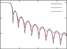
where δθ is the beam angular divergence. The divergence of the incident beam is usually determined by the two collimation slits if the beam is smaller than the effective width of the sample seen by the neutron beam, or by the first slit and the sample itself if the sample is small enough to be totally illuminated by the neutron beam. The experimental reflectivity is then the calculated reflectivity convoluted by a resolution function whose width is given by δQ. Experience shows that Gaussian function works well to reproduce the resolution effects. In Fig. 9.10 the reflectivity is calculated for a perfect instrument and by taking into account the effects of angular divergence and wavelength spread. As can be inferred from Eq. (9.30), angular divergence induces a loss of resolution independent of θ, and wavelength spread degrades the resolution as θ increases. This example shows that, when preparing a reflectometry experiment and depending on the sample under study, a good compromise between intensity and resolution has to be found.
|
1 |
perfect instrument |
|
|
|
|
|
Δθ = 1 mrad |
|
|
|
|
Δλ = 10 % |
|
Reflectivity |
0.01 |
|
|
|
0.0001 |
|
|
|
|
|
|
|
|
|
|
1e−06 |
0.04 |
0.08 |
0.12 |
|
0 |
|||
|
|
Q = 4π/λsin(θ) [Å −1] |
|
|
Fig. 9.10: Effect of δθ and δλ. Comparison between a perfect instrument, an instrumental δθ, and a δλ for a measurement on a 400 A˚ thick Ni layer on Si substrate
Neutron reflectometry |
9.15 |
9.3.4 Data analysis
The method of analysis often used for specular reflection data involves the construction of a model of the multilayer consisting of a series of parallel layers of homogeneous material. Each layer is characterized by a scattering length density ρ and a thickness d, which are used to calculate a model reflectivity profile by means of the recursion method introduced in section 9.2.4 and taking into account the resolution in Q (section 9.3.3). The interfacial roughness or interdiffusion between two consecutive layers, σ, may also be included as described in section 9.2.5. The calculated profile is compared to the measured profile and the quality of the fit is assessed either visually or by using χ2 in the least-square method. By variation of ρ, d and σ in each layer and interface, the calculated profile may be compared with the measured profile until optimum fit to the data is found. Any one profile may not provide a unique solution. This is because only the intensity, and not also the phase of the reflection amplitude is measured. In soft matter, the use of different isotopic contrasts can usually ensure an unambiguous model of the system. Contrast variation relies on the fact that different nuclear isotopes scatter neutrons with different amplitudes, and sometimes, as in the case of protons and deuterons, with opposite phases. By using several combinations of hydrogenated and deuterated materials the reflectivity profile of a layered system can be substantially changed while keeping the same chemical structure. An example where contrast variation is used is given in section 9.5.
9.4Interdiffusion between diblock copolymer layers under annealing
Diblock copolymers are made up of two blocks of different polymerized monomers. Block copolymers are interesting because they can ”microphase separate” to form periodic nanostructures. Microphase separation is a situation similar to that of oil and water. Oil and water are immiscible - they phase separate. Due to incompatibility between the blocks, block copolymers undergo a similar phase separation. Because the blocks are covalently bonded to each other, they cannot demix macroscopically as water and oil. In ”microphase separation” the blocks form nanometer-sized structures. Depending on the relative lengths of each block, several morphologies can be obtained. In diblock copolymers, sufficiently different block lengths lead to nanometer-sized spheres of one block in a matrix of the second (for example PMMA in polystyrene). Using less different block lengths, a ”hexagonally packed cylinder” geometry can be obtained. Blocks of similar length form layers (often called lamellae in the technical literature) [9].
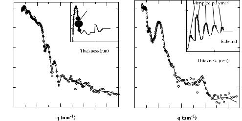
In the study presented in this chapter, a diblock copolymer of the type polystyrene - polybutylmetacrylate (PS-PBMA), with similar lengths of the two blocks, has been deposited on a substrate by spin-coating, forming a self-organized multilayer of a fixed thickness parallel to the surface. The initial system consists in a layer of partially deuterated PS-PBMA copolymer deposited on a trilayer of totally hydrogenated copolymer. The reflectivity of the system is shown on the left picture of Fig. 9.11. The numerical fit shows a large index at the top of the system corresponding to the deuterated copolymer. The system has then been annealed for 12 hours at 400 K and then remeasured (right picture of Fig. 9.11). On this reflectivity curve, one can observe a clear “Bragg” peak at the position q1 = 0.11 nm−1, and a second
9.16 |
E. Kentzinger |
one at q2 = 0.29 nm−1. |
This indicates the diffusion of the deuterated polymer to the inner |
layers. Since the diblock copolymers are ordered in multilayers, a periodic variation of the index appears (see insert in Fig. 9.11), whose period is approximately given by 2π/(q2 − q1). (After [10])
Fig. 9.11: Left: Reflectivity of a quadrilayer consisting in a partially deuterated PS-PBMA copolymer layer deposited on a trilayer of totally hydrogenated polymer. Right: Reflectivity of the quadrilayer after annealing for 1 hour at 115 C. (After [10]). Measurements performed on the time-of-flight reflectometer EROS at the Laboratoire Leon´ Brillouin [11]
9.5Structural characterization of sparsely tethered bilayer lipid membranes
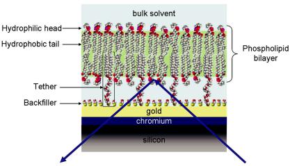
All cells are enclosed by biological membranes that define their boundaries and regulate their interactions with the environment. The biological membrane consists of assemblies of lipid and protein molecules. The lipid molecules form a continuous double layer, or bilayer, which acts as a barrier to water-soluble molecules and provides the framework for the incorporation of the protein molecules. The intrinsic complexity of the cell membrane system often precludes direct access to these features, thus driving the development of simpler model systems that are more amenable to a detailed characterization. One generic approach involves supports for the stabilization of biomimetic membranes. The work shown here focuses on a membrane system, illustrated in Fig. 9.12, that is chemically tethered to a gold support through a tether lipid.
Tethered membranes are systems designed for the incorporation of membrane-associated proteins. In order to be useful as a biomembrane model, such membranes need to retain their fluid in-plane organization and at the same time remain separated from the supporting solid interface by a molecularly thin hydration layer. In order to create space for hydration, the tether lipid
Neutron reflectometry |
9.17 |
is co-adsorbed with a smaller “backfiller” molecule (see Fig. 9.12). The resulting “sparselytethered membrane” has been characterized by ellipsometry, electrochemical impedance spectroscopy and neutron reflectometry [12].
Fig. 9.12: Sparsely tethered biomimetic membrane. The arrows show the geometry of the neutron reflection experiment: the neutrons hit the sample from the side of the silicon substrate.
Neutron reflection is uniquely capable of characterizing in molecular detail the resulting membrane structure, particularly with respect to the thin hydration layer. Fig. 9.13 shows data sets measured on the system discussed above in three distinct solvent contrasts (pure D2O, pure H2O and a H2O/D2O mixture with SLD 4 × 10⁻⁶ A˚ −2 called CM4). The three measurements used the same sample, with the exchange of the isotopically distinct water solutions performed in-situ, and were co-refined on the assumption that the sample is identical except for the distinct solvent contrasts. As is evident from the differences in the SLD profiles, the spacer region containing the tethers is highly hydrated while the bilayer membrane covers the substrate homogeneously: only a minimal hydration of the inner leaflet is present. Such a system thus constitutes a biomimetic membrane that is very well suited to understand the interaction between lipid bilayer and membrane proteins [13,14].
The top graph of Fig. 9.13 shows measurements performed on a system with a molar proportion of tether to backfiller at the gold surface equal to 30 to 70 and the bottom graph shows measurements performed with this proportion equal to 15 to 85. The SLD profiles show that the aqueous reservoir for the system containing 30 % of tether at the gold surface is 21 A˚ thick, the one for the system containing 15 % of tether being slighlty thinner, i.e. 19 A˚ thick. This slight difference in thicknesses is revealed by slight shifts in the positions of the intensity maxima and minima in the region of scattering wave vectors around Qz = 0.2 A˚ −1. This comparison gives an idea of the high resolution of the neutron reflection technique.

9.18 |
E. Kentzinger |
Fig. 9.13: Neutron reflectometry on sparsely tethered bilayer lipid membranes. The two graphs represent measurements performed on two different samples with two different molar proportions of tether and backfiller molecules anchored at the gold surface. Top graph: 30 % of tether. Bottom graph: 15 % of tether. Those measurements were performed on the Advanced Neutron Diffractometer/Reflectometer (AND/R) [15] at the NIST Center for Neutron Research (NCNR).
9.6 Conclusion and outlook
This chapter has given an overview of neutron reflectometry as a tool for the investigation of surfaces and interfaces. We have presented a formalism which makes it possible to describe the specular reflectivity on non-magnetic systems. Neutron reflectivity is especially suited for polymer and magnetic thin film systems. This has been illustrated with two examples. The formalism of neutron reflectometry for the investigation of the magnetic moment orientations in magnetic multilayers is presented in the next chapter of this book, together with several application examples.
Neutron reflectometry |
9.19 |
Recently, the neutron reflectometry technique has been extended to study nuclear and magnetic structures in the sample surface. At grazing incidence, it is possible to distinguish three scattering geometries: specular reflection, scattering in the incidence plane of the neutrons (off-specular scattering) and scattering perpendicular to the incidence plane (grazing incidence SANS). These different scattering geometries probe different mesoscopic length scales and directions in the sample surface [16–19].