References
[1]A special issue of Langmuir covers a broad range of applications of this technique for the characterization of surfaces and interfaces in the fields of soft matter and biology:
Lamgmuir 25(7), (2009).
[2]P. Gr¨unberg, J. Phys. Condens. Matter 13, 7691 (2001).
[3]M. Born and E. Wolf, Principles of Optics (Pergamon Press, Oxford, 1989).
[4]L.G. Parratt, Phys. Rev. 95, 359 (1954).
[5]S.K. Sinha, E.B. Sirota, S. Garoff, H.B. Stanley, Phys. Rev. B 38:4, 2297 (1988).
[6]L. N´evot, P. Croce, Rev. de Phys. Appl. 15, 761 (1980).
[7]http://www.jcns.info/MARIA new
[8]http://neutrons.ornl.gov/instruments/SNS/MR/
[9]I.W. Hamley, The Physics of Block Copolymers (Oxford University Press, Oxford, 1998).
[10]C. Fermon, F. Ott, A. Menelle: “Neutron Reflectometry” in J. Daillant, A. Gibaud (eds),
X-Ray and Neutron Reflectivity: Principles ans Applications (Springer, Berlin, 1999).
[11]http://www-llb.cea.fr/en/fr-en/spectros p.php
[12]F. Heinrich, T. Ng, D.J. Venderah, P. Shekar, M. Mihailescu, H. Nanda, M. L¨osche, Langmuir 25, 4219 (2009).
[13]D.J. McGillivray, G. Valincius, F. Heinrich, J.W.F. Robertson, D.J. Vandrah, W. FeboAyala, I. Ignatjev, M. L¨osche, J.J. Kasianowicz, Biophysical Journal 96:4, 1547 (2009).
[14]S.A.K. Datta, F. Heinrich, S. Raghunandan, S. Krueger, J.E. Curtis, A. Rein, H. Nanda, J. Mol. Biol. 406, 205 (2011).
[15]J.A. Dura, D.J. Pierce, C.F. Majkrzak, N.C. Maliszewskyi, D.J. McGillivray, M. L¨osche, K.V. O’Donovan, M. Mihailescu, U. Perez-Salas, D.L. Worcester and S.H. White, Rev. Sci. Instrum. 77, 074301 (2006).
[16]P. M¨uller-Buschbaum, E. Maurer, E. Bauer, R. Cubitt, Langmuir 22, 9295 (2006).
[17]E. Kentzinger, H. Frielinghaus, U. R¨ucker, A. Ioffe, D. Richter and Th. Br¨uckel, Physica B 397, 43 (2007).
[18]E. Kentzinger, U. R¨ucker, B. Toperverg, F. Ott and Th. Br¨uckel, Phys. Rev. B 77, 104435 (2008).
[19]D. Korolkov, P. Busch, L. Willner, E. Kentzinger, U. R¨ucker, A. Paul, H. Frielinghaus, and Th. Br¨uckel, submitted to J. Appl. Cryst. (2011)
Neutron reflectometry |
9.21 |
Exercises
In the following the nuclear scattering length densities (in 10−6 A˚ −2) of several elements are displayed:
Cu: 6.53; Ag: 3.5; Si: 2.15; Au: 4.5
E9.1 Reflection and transmission by a flat substrate
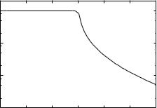
The following figure shows the neutron reflectivity from a flat substrate.
1 |
|
|
|
|
|
|
0.1 |
|
|
|
|
|
|
0.01 |
|
|
|
|
|
|
0.001 |
0.05 |
0.1 |
0.15 |
0.2 |
0.25 |
0.3 |
0 |
|
|
|
Q [nm-1] |
|
|
|
Fig. 9.14: Reflectivity from a substrate.
•Determine the element of which this substrate is made of
•Explain why the amplitude of the wave transmitted in the substrate is equal to 2 at an angle of incidence equal to the critical angle of total reflection
E9.2 Layers on substrate
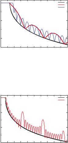
The figure below shows two simulations of reflectivity from a Cu layer deposited on Ag substrate. Determine for both cases (red and blue curves) the thickness of the Cu layer.
1 |
|
|
|
|
|
Substrate only |
|
|
|
|
|
|
|
|
|
Cu on Ag |
|
|
|
|
|
|
|
|
|
Cu on Ag |
|
|
0.01 |
|
|
|
|
|
|
|
|
|
|
0.0001 |
|
|
|
|
|
|
|
|
|
|
0 |
0.1 |
0.2 |
0.3 |
0.4 |
0.5 |
0.6 |
0.7 |
0.8 |
0.9 |
1 |
|
|
|
|
|
Q [nm-1] |
|
|
|
|
|
Fig. 9.15: Layer of Cu on Ag substrate
In the next figure, the reflectivity from a [Cu/Au]×n multilayer is depicted. Determine the [Cu/Au] thickness, the total thickness of the multilayer and the number n of bilayers the multilayer is composed of.
1 |
|
|
|
|
|
Substrate only |
|
|
|
|
|
|
|
|
Cu/Au multilayer |
|
|
0.01 |
|
|
|
|
|
|
|
|
|
|
0.0001 |
|
|
|
|
|
|
|
|
|
|
1e-06 |
0.2 |
0.4 |
0.6 |
0.8 |
1 |
1.2 |
1.4 |
1.6 |
1.8 |
2 |
0 |
|
|
|
|
|
Q [nm-1] |
|
|
|
|
|
Fig. 9.16: Cu/Au multilayer on Ag substrate
10 Magnetic Nanostructures
U. Rücker
Jülich Centre for Neutron Science 2
Forschungszentrum Jülich GmbH
Contents |
|
10.1 |
Introduction....................................................................................... |
2 |
10.2 |
Why neutrons are useful for investigating magnetic |
|
|
nanostructures................................................................................... |
5 |
10.3 |
Specular reflectivity of polarized neutrons..................................... |
6 |
10.4 |
Layer-by-layer magnetometry......................................................... |
9 |
10.5 |
Vector magnetometry ..................................................................... |
11 |
References .................................................................................................. |
19 |
Exercises..................................................................................................... |
20 |
________________________
Lecture Notes of the JCNS Laboratory Course Neutron Scattering (Forschungszentrum Jülich, 2012, all rights reserved)
10.1 Introduction
The physical properties of a layered structure of nanometer size, as it is shown schematically in Fig. 10.1, differs from the bulk properties of the constituents. There are several origins of new effects due to miniaturization:
The ratio between surface and volume is much higher than in bulk. Therefore, the amount of atoms with reduced coordination is significant and can change the crystalline structure as well as the electronic structure of the whole layer. Boundary conditions, e.g. for the magnetic induction B become important, introducing shape anisotropies. The magnetization tends to align along the long edges of the magnetic nanostructure because the dipolar fields are smaller then.
At the interface between two layers, the electronic structures and the crystal lattices have to be matched, which leads to structural stress, interfacial disorder and electronically to charge transfer (e.g. a Shottky barrier in semiconductor heterostructures) or splitting of the layers’ bandstructures.
Nanostructures can be prepared in several dimensions: thin films with a thickness in the nm range are 2D nanostructures, stripes with thickness and width in the nm range are 1D nanostructures and dots or nanoparticles with all three dimensions in the nm range are 0D nanostructures. The dimension number indicates, in how many directions the dimension remains macroscopic.
Magnetic nanostructures are nanostructures which contain at least one magnetic constituent. Typical systems are layered structures with ferromagnetic and nonmagnetic layers or arrays of ferromagnetic dots on a nonmagnetic substrate. The interesting aspect of magnetic nanostructures is the fact that two ferromagnetic (FM) layers with a nonmagnetic (NM) spacer in between have a connection between their electronic systems across the spacer layer. This connection influences as well the magnetic behaviour as the electron transport through the system.
Fig. 10.1: Sketch of a layered structure of two materials
Magnetic Nanostructures |
10.3 |
Co
Co
Co
Co
Fig. 10.2: Oscillating interlayer coupling as a function of interlayer thickness
The first phenomenon found in magnetic layered structures has been the oscillating magnetic interlayer coupling in FM / NM / FM trilayer structures. Depending on the NM interlayer thickness, the magnetizations of the two FM layers tend to align parallel or antiparallel to each other [1]. It turned out that the coupling is mediated by electronic states in the NM interlayer close to the Fermi surface [2]. The oscillation period of the coupling is related to the length of the wavevector of the electrons at the Fermi surface, as is sketched in Fig. 10.2.
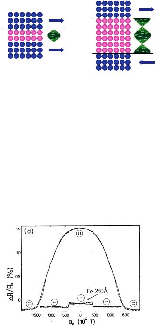
Subsequently, the most important discovery followed, the Giant Magnetoresistance Effect (GMR) [3] [4]. For this discovery, P. Grünberg and A. Fert were honoured with the Nobel Prize for Physics 2007. They have found out that the resistivity of a layered structure containing more than one ferromagnetic layer depends on the mutual orientation of the magnetization directions, see Fig. 10.3. They used the antiferromagnetic coupling in Fe / Cr / Fe trilayer structures to be able to influence the mutual orientation of the magnetization of the Fe layers by changing the applied magnetic field.
Fe/Cr/Fe
Fig. 10.3: Giant Magnetoresistance effect in an Fe / Cr / Fe trilayer compared to the anisotropic magnetoresistance effect in a single Fe layer [3]
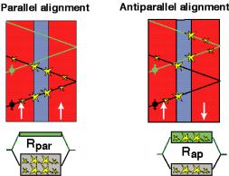
Fig. 10.4: Different matching of the bandstructure between ferromagnetic and nonmagnetic layers changes the resistivity for the different spin channels
It turns out that the resistivity is highest in the case of antiparallel alignment of the two magnetization directions. This effect is much stronger and much more sensitive to changes in the magnetization direction of each ferromagnetic layer than the anisotropic magnetoresistance effect in single ferromagnetic layers, which was known before. The microscopic origin of the GMR effect is the matching between the spin-split bandstructures of the two ferromagnetic layers. The conductivity of the entire structure is the sum of the conductivities for the two spin channels. As the Fermi surface is different for the two spin channels, the matching between the FM and the NM layer is different.
As shown in Fig. 10.4, in the case of parallel alignment, the scattering probability of a conduction electron is the same at both interfaces. For one spin channel, the scattering probability is high while for the other it is low. The conductivity is then dominated by the spin channel with the smaller scattering probability. The resistivity of the entire structure, which can be described as a parallel wiring of the two resistors for the two spin channels, is small.
In the case of antiparallel alignment, the scattering probability for each spin channel is high in one of the FM layers. This results in a relatively low conductivity for both spin channel, so that the resulting resistivity is much higher compared to the case of parallel magnetization.
As GMR structures are easy to prepare and easy to use, the sensor technology based on this effect quickly became standard in the readout system of computer harddisks and many other applications. Today, it has been replaced by Tunneling Magnetoresistance (TMR), where the nonmagnetic interlayer is insulating and electrons travel across this tunneling barrier while preserving their spin state. Then, the height of the tunneling barrier depends on the spin of the electron and the magnetization direction of both ferromagnetic layers. A detailed overview over the field of spin transport in layered systems is given in Ref. [5].
Magnetic Nanostructures |
10.5 |
10.2Why neutrons are useful for investigating magnetic nanostructures
For the investigation of magnetism, many methods are well known. In most cases the magnetization of a sample is measured. A different, but more indirect approach is the measurement of spin-dependent bandstructures by absorption and photoemission spectroscopy of polarized light / x-rays.
The first (and oldest) approach is to measure the integral magnetization of a sample by classical magnetometry, e.g. by using a Vibrating Sample Magnetometer (which measures the induction when moving the magnetic sample in a coil), a Faraday balance (which measures the force on the magnetic sample in a field gradient), or more recently a SQUID magnetometer (which measures the magnetic flux inside a superconducting loop). In case of magnetic nanostructures, the small signal coming from the nanostructure is always superimposed by the signal from the substrate which is typically 10000 times larger in volume. Even if the nanostructure is ferromagnetic and the substrate only diamagnetic, the correction due to the substrate is in most cases much stronger then the signal itself.
Better adapted to thin structures are methods that are surface sensitive. The magnetooptical Kerr effect (MOKE) measures magnetization with polarized light reflected from a magnetic surface. Due to the magnetization of the sample the polarization direction of the light is modified. This method is surface sensitive in the range of the penetration depth of the light used (typically some 10 nanometers). At synchrotron x-ray sources one can use X-ray Magnetic Circular Dichroism (XMCD). The energy dependence of the absorption of circular polarized (soft) x-rays is measured at the absorption edges of the magnetic materials. Again, the information is integrated over the penetration depth of the x-rays used, but it is element specific due to the choice of the x-ray energy in resonance with the magnetic orbitals of a certain element.
Magnetic domains can be imaged using e.g. Magnetic Force Microscopy (surface sensitive, measuring the stray fields above the sample), Lorentz microscopy (the transmission of electrons through a very thin sample is observed; due to the Lorentz forces the electrons are deviated according to the magnetization strength and direction), or Kerr microscopy (observing the MOKE using an optical microscope; again it integrates over the penetration depth of the light, with the lateral resolution of the optical microscope). Photoemission electron microscopy (PEEM) with soft x-rays can give an overview about the density of certain electronic states with a lateral resolution in the nanometer range and time resolution down to nanoseconds. In combination with XMCD, XMCD-PEEM can visualize the evolution of magnetic domains under variable magnetic fields. But again, the depth resolution is only determined by the penetration depth and the element specific absorption of the x-rays.
What is missing is a method that can access the magnetism of buried layers using the depth information. Here, we need a probe that is sensitive to magnetic fields while having a spatial resolution (at least in depth) in the nm regime. Cold neutrons have a wavelength appropriate for resolving nm length scales and they carry a spin that interacts with the magnetic fields. For most of the magnetic investigations, the neutron’s
spin has to be prepared in a certain state, so we use polarized neutrons for the investigation of magnetic nanostructures.
Polarized neutron reflectometry with polarization analysis is a method for depthresolved investigation of magnetic layered structures; I will introduce this method in the following chapter. Together with the analysis of off-specular scattering, lateral structures in the μm range can be investigated, allowing to access magnetic domains in buried layers. Polarized SANS reveals information about magnetic structures in the nm range perpendicular to the beam direction, while polarized GISANS (Grazing Incidence Small Angle Neutron Scattering) combines the possibilities of both methods and allows to access lateral magnetic structures in the nm range in buried layers.
10.3 Specular reflectivity of polarized neutrons
In the previous lecture, you have learned about specular reflectivity of neutrons on layered structures with nuclear scattering contrast. For the investigation of magnetic layered structures, we have to remind that the neutron is a spin ½ particle and therefore interacts with the magnetic induction B.
To treat the neutron’s spin properly, we have to work with wave functions in the 2- dimensional quantum mechanical spin space, where the usual space-dependent functions, e.g. the potential, become operators on the neutron’s spin.
In analogy to eq. (9.2), the potential of a homogeneous magnetic material can be separated into two parts
ˆ |
N ˆ |
ˆ M |
(10.1) |
Vl |
Vl 1 |
Vl |
where V1N is the nuclear interaction from eq. (9.2), and 1ˆ is the unity operator, which does not affect the spin state, so that the nuclear interaction is described independently on the neutron’s spin. The magnetic dipole interaction is described by the operator
Vˆ lM n ˆ Bl which is a scalar product of the neutron magnetic moment operator
n ˆ and the magnetic induction Bl inside the material.
For the description in coordinates, we need to define a coordinate system which is convenient to describe the experiment. Typically, the magnetic field H is applied in the plane of the sample. We choose this direction to be the x-direction of the coordinate system H = Hex and also as the quantization axis for the neutron spin. Under this assumption, the spin operator ˆ ( x , y , z )is the following:
x |
1 |
0 |
y |
0 |
1 |
z |
0 |
i |
(10.2) |
|
|
|
|
|
|
|
0 |
1 |
|
1 |
0 |
|
i 0 |
|
Magnetic Nanostructures |
10.7 |
In analogy to chapter 9.2, the Schrödinger equation can be solved in coordinate and spin space, where the eigenvectors  and
and  of the operator ˆ b0 x with the
eigenvalues +1 and -1, respectively, define states of the neutron with “spin up” and “spin down”. The solution of the Schrödinger equation is the neutron wave function(r) , which is again a linear combination of those two spin states.
|
|
|
|
|
|
|
|
|
|
|
(r) |
|
|
|
|
|
|
(r) |
|
|
|
|
(r) |
|
|
(r) |
|
|
|
|
(10.3) |
|
|
|
|
|
|
|
|
(r) |
|
After some calculation which you can find in Ref [6] we end up with a set of two coupled one-dimensional linear differential equations for every layer, which are the analogue to equation (9.8).
l (z) kzl2 |
4 ( lN lM mxl ) l (z) 4 lM myl l (z) 0 |
(10.4) |
l (z) kzl2 |
4 ( lN lM mxl ) l (z) 4 lM myl l (z) 0 |
(10.5) |
In this formulae, you find the nuclear scattering length density N that you know from eq. (9.3) together with its magnetic analogon M , the magnetic scattering length density. It is proportional to the net magnetization M of the material. In case of a ferromagnetic material, the magnetization vector M typically is aligned in some direction, which is described by the unit vector m = M / M.
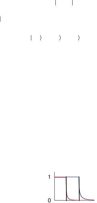
Now, we can have a closer look at the different terms in equation (10.4) and (10.5). As Non-Spinflip (NSF) interaction, one finds in (10.4) for spin + (“spin up”) the sum of the nuclear interaction and the magnetic interaction with the magnetization along the quantization direction and in (10.5) for spin – (“spin down”) the difference. In case of a magnetically saturated layer (all the magnetization is aligned with the external field), the scattering length density for spin + neutrons is enhanced and for spin – neutrons is reduced compared to the nonmagnetic case.
R- R+
c- c+
Fig. 10.5: The total reflection angle c of the surface of a magnetized material is different for both spin directions