Fig. 10.15: Polarized neutron reflectivity and offspecular scattering for two AF-coupled
[Fe / Cr]N multilayers with N = 7 (top) and N = 19 (bottom) in
remanence field of 5 mT. Indicated are the AF superstructure Bragg peaks of order ½ in the NSF channels of the [Fe / Cr]7 system (1) and in the SF channels of the [Fe / Cr]19 system (2).
Magnetic Nanostructures |
10.19 |
References
[1]P. Grünberg, R. Schreiber, Y. Pang, M.B. Brodsky, and H. Sowers, Phys. Rev. Lett. 57 (1986), 2442
[2]P.H. Dederichs, “Interlayer Exchange Coupling“, chapter C 3 in “Magnetism goes Nano“, 36th IFF Spring School, Forschungszentrum Jülich, series Matter and Materials, Vol. 26 (2005)
[3]G. Binasch, P. Grünberg, F. Saurenbach, and W. Zinn, Phys. Rev. B 39 (1989), 4828
[4]M.N. Baibich, J.M. Broto, A. Fert, F. Nguyen Van Dau, F. Petroff, P. Etienne, G. Creuzet, A. Friedrich, and J. Chazelas, Phys. Rev. Lett. 61 (1988), 2472
[5]D.E. Bürgler, “Spin-Transport in Layered Systems“ , chapter E 5 in “Magnetism goes Nano“, 36th IFF Spring School, Forschungszentrum Jülich, series Matter and Materials, Vol. 26 (2005)
[6]U. Rücker, E. Kentzinger, “Thin Film Systems: Scattering under Grazing Incidence”, chapter D4 in “Probing the Nanoworld”, 38th IFF Spring School, Forschungszentrum Jülich, series Matter and Materials, Vol. 34 (2007)
[7]A. Paul, E. Kentzinger, U. Rücker, D.E. Bürgler, and P. Grünberg, Phys. Rev. B 70 (2004), 224410
[8]E. Josten, U. Rücker, S. Mattauch, D. Korolkov, A. Glavic, and Th. Brückel, J. Phys: Conf. Ser. 211 (2010), 012023
Exercises
E10.1 Magnetic contrast
We measure the polarized neutron reflectivity of a [Ni2Fe / Pt]N multilayer structure in magnetic saturation. The Ni2Fe alloy is ferromagnetic.
a)Calculate the nuclear and magnetic scattering length densities for the two constituents of the multilayer:
|
Ni |
Fe |
Pt |
density [g/cm³] |
8.90 |
7.86 |
21.4 |
atomic weight [g/mol] |
58.71 |
55.85 |
195.09 |
nuclear scattering length [1E-14 m] |
1.03 |
0.954 |
0.95 |
magnetic scattering length density |
1.52 |
5.12 |
0 |
[1E-6 Å-2] |
|
|
|
If you do not manage to calculate the values properly, you may continue with the tabulated values of the nuclear scattering length densities: Ni: 9.41E-6 Å-2, Fe: 8.09E-6 Å-2, Pt: 6.29E-6 Å-2.
b)Which of the 5 reflectivity curves presented below is the one measured on this alloy? Think about the critical angle (has to do with the highest scattering length density in all layers) and the contrast between adjacent layers (influences the height of the diffraction peaks) for both spin directions parallel (R+ +) and antiparallel (R– – ) to the applied magnetic field (saturation!).
|
100 |
|
|
|
|
|
100 |
|
|
|
|
|
|
100 |
|
|
|
|
|
|
|
|
|
|
R++ |
|
|
|
|
|
R++ |
|
|
|
|
|
|
R++ |
|
|
|
|
|
|
R- - |
|
|
|
|
|
R- - |
|
|
|
|
|
|
R- - |
|
Reflectivity |
10-2 |
|
|
|
|
Reflectivity |
10-2 |
|
|
|
|
|
Reflectivity |
10-2 |
|
|
|
|
|
|
|
|
|
|
|
|
|
|
|
|
|
|
|
|
|
|
|
10-4 |
|
|
|
|
|
10-4 |
|
|
|
|
|
|
10-4 |
|
|
|
|
|
|
|
a) |
|
|
|
|
|
b) |
|
|
|
|
|
|
c) |
|
|
|
|
|
10-6 |
20 |
40 |
60 |
80 |
100 |
10-6 |
20 |
40 |
60 |
80 |
100 |
|
10-6 |
20 |
40 |
60 |
80 |
100 |
|
0 |
0 |
|
0 |
|
|
|
|
[mrad] |
|
|
|
|
|
[mrad] |
|
|
|
|
|
|
[mrad] |
|
|
|
100 |
|
|
|
|
|
100 |
|
|
|
|
|
|
|
|
|
|
|
|
|
|
|
|
|
R++ |
|
|
|
|
|
R++ |
|
|
|
|
|
|
|
|
|
|
|
|
|
R- - |
|
|
|
|
|
R- - / 10 |
|
|
|
|
|
|
|
|
Reflectivity |
10-2 |
|
|
|
|
|
Reflectivity |
10-2 |
|
|
|
|
|
|
|
|
|
|
|
|
|
|
|
|
|
|
10-4 |
|
|
|
|
|
|
10-4 |
|
|
|
|
|
|
|
d) |
|
|
|
|
|
|
e) |
|
|
|
|
|
10-6 |
20 |
40 |
60 |
80 |
100 |
|
10-6 |
20 |
40 |
60 |
80 |
100 |
|
0 |
|
0 |
|
|
|
|
[mrad] |
|
|
|
|
|
|
[mrad] |
|
|
Magnetic Nanostructures |
10.21 |
c)The other 4 curves have been measured on different samples. Which curve belongs to which sample?
I.The sum of nuclear and magnetic scattering length density of the magnetic layers is equal to the nuclear scattering length density of the nonmagnetic
layers
II.The sample contains an additional nonmagnetic layer with a scattering length density higher than the sum of the magnetic and nuclear scattering length
densities of Ni2Fe on top of the [Ni2Fe / Pt]N multilayer III. No layer is magnetic
IV. The nuclear scattering length density of the nonmagnetic layers is somewhere between the sum and the difference of nuclear and magnetic scattering length density of the magnetic layers
E10.2 Vector magnetometry
The following figures show polarized neutron reflectivity measurements with polarization analysis from a ferromagnetic single layer on a nonmagnetic substrate. Find out which figure belongs to which magnetization state:
I. The sample is magnetized perpendicular to the field direction II. The sample is magnetized parallel to the field direction
III. The magnetization of the sample is inclined by 45° against the field direction IV. This set of curves is wrong. (Why?)
|
100 |
|
|
|
R++ |
|
|
100 |
|
|
|
R++ |
|
|
|
|
|
|
|
|
|
|
|
|
|
|
|
|
|
|
R- - / 10 |
|
|
|
|
|
|
R- - / 10 |
|
|
-2 |
|
|
|
R+- / 100 |
|
|
-2 |
|
|
|
R+- / 100 |
|
|
10 |
|
|
|
R-+ / 1000 |
|
|
10 |
|
|
|
R-+ / 1000 |
|
Reflectivity |
10-4 |
|
|
|
|
|
Reflectivity |
10-4 |
|
|
|
|
|
|
|
|
|
|
|
|
|
|
|
|
|
|
10-6 |
|
|
|
|
|
|
10-6 |
|
|
|
|
|
|
|
a) |
|
|
|
|
|
|
b) |
|
|
|
|
|
10-8 |
|
|
|
|
|
|
10-8 |
|
|
|
|
|
|
0 |
20 |
40 |
60 |
80 |
100 |
|
0 |
20 |
40 |
60 |
80 |
100 |
|
|
|
|
[mrad] |
|
|
|
|
|
|
[mrad] |
|
|
|
100 |
|
|
|
R++ |
|
|
100 |
|
|
|
R++ |
|
|
|
|
|
|
|
|
|
|
|
|
|
|
|
|
|
|
R- - / 10 |
|
|
|
|
|
|
R- - / 10 |
|
|
-2 |
|
|
|
R+- / 100 |
|
|
-2 |
|
|
|
R+- / 100 |
|
|
10 |
|
|
|
R-+ / 1000 |
|
|
10 |
|
|
|
R-+ / 1000 |
|
|
|
|
|
|
|
|
|
|
|
|
|
Reflectivity |
10-4 |
|
|
|
|
|
Reflectivity |
10-4 |
|
|
|
|
|
|
|
|
|
|
|
|
|
|
|
|
|
|
10-6 |
|
|
|
|
|
|
10-6 |
|
|
|
|
|
|
|
c) |
|
|
|
|
|
|
d) |
|
|
|
|
|
10-8 |
|
|
|
|
|
|
10-8 |
|
|
|
|
|
|
0 |
20 |
40 |
60 |
80 |
100 |
|
0 |
20 |
40 |
60 |
80 |
100 |
|
|
|
|
[mrad] |
|
|
|
|
|
|
[mrad] |
|
|
11 Inelastic Neutron Scattering
R. Zorn
Julich¨ Centre for Neutron Science 1
Forschungszentrum Julich¨ GmbH
Contents |
|
11.1 |
Introduction |
2 |
11.2 |
Theory |
2 |
|
11.2.1 Kinematics of neutron scattering . . . . . . . . . . . . . . . . . . . . . . . . |
2 |
|
11.2.2 Scattering from vibrating atoms . . . . . . . . . . . . . . . . . . . . . . . . |
3 |
|
11.2.3 Scattering from diffusive processes . . . . . . . . . . . . . . . . . . . . . . |
8 |
11.3 |
Instrumentation |
17 |
|
11.3.1 Triple axis spectrometer . . . . . . . . . . . . . . . . . . . . . . . . . . . . |
17 |
|
11.3.2 Time-of-flight spectrometer . . . . . . . . . . . . . . . . . . . . . . . . . . |
18 |
|
11.3.3 Backscattering spectrometer . . . . . . . . . . . . . . . . . . . . . . . . . . |
20 |
|
11.3.4 Neutron spin echo spectrometer . . . . . . . . . . . . . . . . . . . . . . . . |
22 |
References |
25 |
Exercises |
27 |
Lecture Notes of the JCNS Laboratory Course Neutron Scattering (Forschungszentrum Julich,¨ 2011, all rights reserved)
11.1 Introduction
One of the most important benefits of neutron scattering is the possibility to do inelastic scattering and by this way gain insight into the dynamics of materials as well as the structure. Neutrons tell us where the atoms are and how they move [1]. Although this feature is shared with inelastic x-ray scattering and dynamic light scattering, there is still a considerable range of slow dynamics in molecular systems which can be studied exclusively by inelastic neutron scattering.
This lecture can only present a short glimpse on the theoretical foundations and instrumental possibilities of inelastic neutron scattering. For those who are interested in more details, several textbooks can be recommended [2–6]. Also supplementary information on correlation functions [7] and Fourier transforms [8] may be found in earlier editions of this school.
Q
k'
 2θ
2θ
k
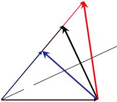
Fig. 11.1: Definition of the scattering vector Q in terms of the incident and final wave vectors k and k . The black (isosceles) triangle corresponds to elastic scattering. The blue and red ones correspond to inelastic scattering with energy loss or gain of the scattered neutron, respectively.
11.2 Theory
11.2.1 Kinematics of neutron scattering
Up to this lecture it has always been assumed that the wavelength (or wave vector, or energy) of the neutrons is the same before and after scattering. The defining quality of inelastic neutron scattering is that this is not anymore the case. The neutrons may lose or gain energy in the collision with the nuclei implying that k = k. This implies that Q now does not anymore result from the isosceles construction drafted in black in Fig. 11.1 but from scattering triangles as those in blue and red. Application of the cosine theorem leads to the following expression for

Inelastic Neutron Scattering |
|
|
|
|
|
|
|
|
|
|
|
|
|
|
11.3 |
Q in the inelastic situation: |
|
|
|
|
|
|
|
|
|
|
|
|
|
|
|
|
|
|
|
|
|
|
|
|
|
|
|
|
(11.1) |
Q = |
k2 + k 2 − 2kk cos(2θ) |
|
|
|
|
) |
|
|
|
|
|
|
|
|
|
|
|
|
|
|
= |
|
λ2 + |
|
− |
4λ |
|
|
|
|
cos(2θ) . |
(11.2) |
|
λ2 + |
|
|
|
|
8π2 |
2mω |
|
|
π |
|
4π2 |
2mω |
|
Note that there is a fundamental difference to the simpler expression for elastic scattering, |
|
|
|
|
Qel |
= |
4π |
sin θ , |
|
|
|
(11.3) |
|
|
|
|
|
|
|
|
|
|
|
|
|
|
λ |
|
|
|
|
|
|
|
used in the preceding lectures. Q now also depends on the energy transfer ω implying that Q is not anymore constant for a single scattering angle. Fig. 11.2 shows the magnitude of this effect for typical parameters of a neutron scattering experiment. It can be seen that it is by no means negligible for typical thermal energies of the sample even at temperatures as low as 100 K.
The other fundamental difference to elastic scattering to be considered is that the total scattering cross section is not identical anymore to the bound scattering cross section read from tables. In the extreme case of a free nucleus the scattering cross section is reduced to [2]
4πb2
σ = (11.4)
(1 + m/M)2
where M is the mass of the scattering nucleus. It can be seen that in the worst case (scattering from a gas of atomic hydrogen) this is a reduction by 1/4.
11.2.2 Scattering from vibrating atoms
The most important case of inelastic neutron scattering from vibrating atoms is that of scattering from phonons in crystals. In this field, inelastic neutron scattering is the most important tool of research. At first, a short recapitulation of the phonon picture will be presented [9, 10].
As a simplified model for the crystal one can consider a chain of N atoms with mass M regularly spaced by a distance a and connected by springs with the spring constant K. For this system the equations of motion can readily be written down:
d2uj |
= |
|
K |
(uj+1 − 2uj + uj−1) . |
(11.5) |
dt2 |
M |
In addition, it has to be specified what the equations of motions are for the first and the last atom (boundary condition). This is usually done by identifying the left neighbour of the first atom with the last and vice versa, u0 = uN and uN+1 = u1, as in a closed necklace rather than an open chain. This is the most natural choice for large N and called the Born-von-Kar´man´ boundary condition. The equation system (11.5) can be solved by the ansatz
uj (t) = |
Uk(t) exp |
i N |
(11.6) |
|
|
|
kj |
|
|
4 |
|
|
|
|
|
|
3 |
2θ = 170° |
|
|
|
|
|
|
|
|
|
|
] |
|
|
|
|
|
|
−1 |
|
|
|
|
|
|
[Å |
2 |
|
|
|
|
|
Q |
|
|
|
|
|
|
|
1 |
|
|
2θ = 10° |
|
|
|
|
|
kB x 100 K |
|
|
|
0 |
0 |
5 |
10 |
15 |
20 |
|
|
|
|
|
|
E [meV] |
|
|
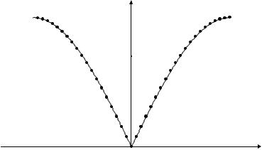
Fig. 11.2: Scattering vectors Q accessed by a neutron scattering experiment with the detector at scattering angles 2θ = 10 . . . 170◦ vs. the energy transfer ω (incident wavelength λ = 5.1 A)˚ . For comparison the thermal energy kBT corresponding to 100 K is indicated by an arrow.
with integer k (k Z). Here, Uk are the normal coordinates and each of them fulfils the equation of motion of a single harmonic oscillator:
ddt2k |
= |
M |
cos |
2N − 1 Uk . |
(11.7) |
2U |
|
2K |
|
πk |
|
By introducing these normal coordinates, the system of differential equations (11.5) can be decoupled into a set of differential equations which can be solved separately. The solutions are
Uk(t) |
= |
Ak exp (iΩkt) with |
|
|
|
|
|
|
|
(11.8) |
|
|
) |
|
|
|
|
|
= 2 |
|
|
sin |
|
. |
|
Ωk |
= |
|
M 1 − cos |
N |
|
N |
(11.9) |
|
|
M |
|
|
|
2K |
2πk |
|
|
K |
|
πk |
|
|
|
|
|
|
|
|
|
|
|
|
|
|
|
|
|
|
|
|
|
|
|
|
|
|
|
|
|
|
|
|
|
|
|
|
|
|
|
|
|
|
|
|
|
The second equation gives a relation between the index of the oscillator k and the frequency. On the other hand, the index determines via equation (11.6) the wavelength of the vibration. One wavelength covers N/k lattice positions, corresponding to λvib = Na/k in actual length. The corresponding wave ‘vector’ is q = 2π/λvib = 2πk/Na1. This implies that there is a relation between the wave vector and the frequency called the dispersion relation (Fig. 11.3):
Ω(q) = 2 |
K |
|
qa |
|
|
|
sin |
|
. |
(11.10) |
M |
2 |
|
|
|
|
|
|
1 As will be seen later, there is a close connection between this lower case q and the scattering vector upper case Q. Nevertheless, they are not the same and care has to be taken not to mix up both q-s.
Inelastic Neutron Scattering |
11.5 |
q
Fig. 11.3: Dispersion relation in a linear chain with N = 40 atoms (Born-von-Karm´an´ boundary condition).
This relation does not contain the number of atoms anymore. For large N the points constituting the curve in Fig. 11.3 will get closer and closer, finally leading to the continuous function (11.10). The individual positions of these points depend on the boundary condition. But because they are getting infinitely dense for N → ∞ the exact boundary conditions do not matter for a large system.
It can be seen that the dispersion relation (11.10) is periodic in q. On the other hand, there are only N normal coordinates necessary to solve the N original equations of motion. This is exactly the number of wave vectors found in a q interval of length 2π/a. The usual choice is −π/a . . . π/a as a representative zone for the dispersion relation.
There are two modifications necessary when considering a real three-dimensional crystal instead of this simplified model: (1) The crystal is periodic in three dimensions. (2) The vibrations are governed by quantum mechanics. The first requirement leads to the consequence that instead of a scalar, one has to use a real wave vector, q → q = (qx, qy, qz) in reciprocal space. The interval defined in Fig. 11.3 changes into a polyhedron called the first Brillouin zone (Fig. 11.4) [9, 10]. It is constructed in the same way as the Wigner-Seitz cell in real space: The Brillouin zone contains all points which are closer to the origin than to any other lattice point. Its surfaces are the bisecting planes between the origin and its neighbours (in reciprocal space).
For every amplitude Ak equation (11.8) gives a valid solution of the equations of motion. This means that in the classical picture the vibrations can have any energy. The quantum mechanical treatment (which is too complex to be treated here in detail) leads to the result that only certain energies with a distance of Ωk are allowed. This quantisation implies that the vibrations can be treated as quasiparticles with the energy Ωk called phonons. The increase of the vibrational amplitude corresponding to an energy change of + Ωk is then seen as a creation, the inverse process as an annihilation of a phonon. Then it makes sense to define q as the momentum of the phonon. In this way the dispersion relation Ω(q) is similar to the relations shown in Fig. 4.2 of lecture 4 for real particles.