Schluesseltech_39 (1)

7Spin Dependent and Magnetic Scattering

R. P. Hermann

Julich¨ Centre for Neutron Science 2

Forschungszentrum Julich¨ GmbH

Contents

Lecture Notes of the JCNS Laboratory Course Neutron Scattering (Forschungszentrum Julich,¨ 2011, all rights reserved)

the spin incoherent scattering can be used as internal calibration for absolute intensity measurements, provided these contributions can be determined separately by polarization analysis, see below and Section 4.

Summarizing, there is thus two sources for incoherent scattering, namely isotopic and spin incoherent scattering, and one might wonder why it is important to differentiate them, as both give rise to isotropic scattering that contains no phase information. A first difference is that it is possible to reduce or enhance isotopic incoherent scattering by isotopic substitution, whereas this is impossible for spin incoherent scattering (unless one were able to align all nuclear spins in the sample which is a daunting but not impossible task [8]). The second difference concerns the effect of the scattering of a neutron by a nucleus with I = 0 on the neutron spin. In order to investigate this effect we need to consider the scattering amplitude and matrix elements for spin dependent scattering

In what follows, we will not explicitly write out the wave vector dependence of these elements. We can use the z projected spin states for the neutron, which we write +| and −| without sacrificing generality. For nuclei with I = 0 we see that A(Q) = Sz|b|Sz = b Sz|Sz . Only the terms with same initial and final neutron spin state are non zero, as +|+ = −|− = 1 and +|− = −|+ = 0. This is not surprising, considering the conservation of total angular momentum.

In the general case, I = 0, angular momentum can be exchanged between the nucleus and the neutron, and the non zero matrix elements are

where NSF and SF denote the spin-flip and non spin-flip scattering amplitude, and Ix, Iy, and Iz are the x, y, and z components of the spin of the nucleus. The derivation of Eq. 7.10 is based on the Pauli spin matrix algebra used for the neutron spin operator, see Appendix A. Note that a flip of the neutron spin occurs only if the nuclear spin is not parallel to the neutron spin, which, as will be discussed later, can be exploited to separate spin incoherent scattering experimentally.

A final question concerns the spin-flip process. As mentioned above, in such a process angular momentum is exchanged. But is there also an exchange in energy? In general this is not the case because the nuclear spin states have all the same energy. However, at low temperature and in some magnetic materials, there might be a splitting in the nuclear spin states through hyperfine interactions. In this case the spin-flip scattering will involve a small transfer in energy between the nucleus and the neutron, and inelastic scattering in the μeV range is observed. This provides an elegant method to measure hyperfine fields [9, 10].

7.3Magnetic Interactions

We will now consider the interaction of the neutron with magnetic fields and thus also the magnetic dipolar moments originating from unpaired electronic spins. For this purpose, the magnetic dipole moment of the neutron μ will be considered. The existence of this purely

magnetic, i.e. non nuclear, interaction of the neutron is extremely useful both in order to manipulate the polarization of a neutron beam and in order to determine the magnetic structure of a material, i.e. the arrangements of the magnetic moments in a sample. Neutron scattering can thus be used as a microscopic magnetometer, with a resolution comparable to the wavelength, that reveals, for example, the onset of magnetic order or the distribution of magnetic moments within nanoparticles.

The dipolar interaction potential of a neutron with the magnetic field is given by VM = −μ · B where B is the magnetic induction, generated e.g. by electrons in a sample or by magnetic coils. The magnetic interaction tends to align the neutron moment within the magnetic induction in order to minimize the interaction energy. However, we know from classical mechanics that the magnetic moment is related to L, the angular momentum as μ = γL, where γ is the gyromagnetic ratio. Thus, the torque G = μ × B, which is equal to the time derivative of the angular

momentum = ˙ , will lead to precession of the angular momentum and of the magnetic

G L

moment and the spin. Accordingly

The gyromagnetic ratio for the neutron, not to be confused with the gyromagnetic factor, is given by

The Larmor precession rate is given by ω = −γB. Note that in Eq. 7.11, the time derivative of the moment is always perpendicular to the moment, which indeed indicates a precession, as only the direction but not the magnitude of the moment changes with time. In contrast, the force exerted on a dipole is given by F = (μ · )B and is zero if the magnetic field is homogeneous.

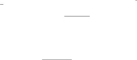
In order to establish how the presence of magnetic moments in a sample leads to magnetic neutron scattering we must now consider the magnetic induction generated by the spin and orbital moment of an electron, see Fig. 7.1. The dipole field of the electronic spin moment,

μe = −2μB · ˆs, is

Fig. 7.1: Left: electronic dipolar field lines and the corresponding induction, BS , in blue, and the field lines and induction, BL, associated with the orbital motion, in red. Right: decomposition of the magnetization vector M in its components parallel and perpendicular to the scattering vector Q.

whereas the magnetic induction generated by the electronic current related tothe orbital motion of the electron is obtained from the Biot and Savard law

The derivation of the scattering law is quite lengthy and the reader is referred to Ref. [1] for

where r0 is the classical electron radius, and the important quantity to consider is the magnetization, i.e. the density of magnetic moments, in reciprocal space, M(Q), which is obtained as the Fourier transformation of the magnetization in real space M(R),

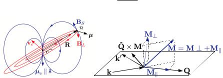
Fig. 7.2: The magnetic field line configuration for M perpendicular, left, and parallel, right, to the scattering vector Q give rise to constructive and destructive interference, respectively.

According to Eq. 7.17, only the component of the magnetization which is perpendicular to the scattering vector contributes to the scattering cross section. The geometrical construction in the right of Fig. 7.1 indicates how this component is obtained as

where ˆ = /Q is the unitary scattering vector. This a priori somewhat surprising scattering

Q Q

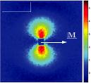
cross section can be understood as illustrated in Fig. 7.2, because the components of any magnetic dipole field parallel to the scattering vector will cancel out. In contrast to spin or isotope incoherent scattering, the magnetic scattering is fundamentally anisotropic with respect to M, and only the component perpendicular to Q is observable. Fig. 7.3 beautifully illustrates this. The intensity is collected on an area detector and is given by the product of the magnetic and nuclear scattering amplitude. Because the sample was magnetized in the horizontal direction,

Fig. 7.3: The product of the magnetic and nuclear scattering amplitude was obtained in a polarized small angle scattering experiment on a collection of magnetized nanoparticles. In the direction parallel to the sample magnetization the magnetic scattering vanishes. (Adapted from Ref. [11]; data obtained at the ILL D22 instrument from the (I+-I−) term in a half-polarized experiment.)

the magnetic scattering vanishes in this direction and intensity is observed only for scattering vectors that have a vertical component.

According to Eqs. 7.17 and 7.18 it is thus in principle possible to determine the magnetization M(R) microscopically, which goes beyond the informations that can be obtained by macroscopic magnetometry measurements.

Before investigating the detailed consequences of the magnetic scattering, it is important to estimate its order of magnitude. If we consider a single unpaired electron with spin s = 1/2 and thus replace the matrix element in Eq. 7.17 by a 1 μB moment, we obtain a scattering length of γnr0/2 = 2.696 fm and a cross section σmag = 0.91 barn. These values are quite comparable to typical nuclear scattering lengths and cross sections. For x-ray scattering the magnetic scattering cross section is between 6 and 9 orders of magnitude smaller than the structural or charge scattering, and although this can be partly mitigated by using resonance scattering techniques, magnetic neutron scattering thus clearly appear at first glance as being at an advantage for investigating magnetism.

We now need to consider the scattering from an ensemble of atoms, or more precisely, here, only their unpaired electrons. First, we neglect the orbital moment (L = 0) and consider pure spin scattering such as for spherically symmetric ions, Fe3+, Mn2+, or ions with fully quenched orbital moment. Ignoring itinerant electrons, we simplify further to an ionic crystal where the electrons are in direct vicinity of the atoms and model these atoms as illustrated in Fig. 7.4. The spin magnetization, i.e. the spin moment density, is

ik

where ˆsik is the spin operator of the kth electron of the ith atom, located at rik in the coordinate system, and at tik with respect to the nucleus. The Fourier transform of the magnetization is

Because the electrons are described by a probability density, the expectation value for the quantum mechanical state must be considered, as well as an averaging over the thermodynamic

Fig. 7.4: The electrons of atom i are located around its position Ri and contribute to the total spin ˆsi.

ensemble representative for the sample. Thus, the spin density, ρs(R), must be Fourier trans-

formed and the magnetic (spin) from factor fm(Q) is obtained as fm(Q) = atom ρs(R)eiQ·RdR and the magnetization is

Ms(Q) = −2μB · fm(Q) · eiQ·Ri · ˆsi (7.22)

i

where we again simplified and considered a single type of atoms in order to factorize the form factor.

Finally, using Eq. 7.17 the differential cross section is given by

In sharp contrast with nuclear scattering, magnetic neutron scattering depends on a form factor in a similar way than for x-ray scattering. This form factor comes about because the scattering no longer occurs on a point-like nucleus but on an extended electronic (spin) cloud, and the larger this cloud is, the faster the form factor drops in reciprocal space. The form factor thus reveals the distribution of the spin and orbital magnetization. Because the unpaired electrons are typically in the outer electronic shells, such as the 3d shell for the first row of transition metal or the 4f shell for the rare earth elements, the magnetic form factor drops faster than for the whole electronic cloud as seen by x-ray scattering, see Fig. 7.5. If an orbital moment is present the magnetic form factor is significantly more complicated, see Appendix B.

Exactly as for spin dependent scattering in the previous section, the spin of the neutron explicitly enters the magnetic scattering cross section. It is thus also important to establish how angular momentum can be exchanged between the sample and the neutron through magnetic scattering, i.e. understand in what conditions the spin of the neutron is flipped by magnetic interactions. For this purpose we consider the magnetic scattering amplitude:

where the sum over α stands for the x, y, and z directions, and σˆα are the Pauli matrices, see Appendix A. Considering all possibilities for the neutron spin state before and after the