Schluesseltech_39 (1)

9Neutron reflectometry

E. Kentzinger

J¨ulich Centre for Neutron Science 2

Forschungszentrum J¨ulich GmbH

Contents

Lecture Notes of the JCNS Laboratory Course Neutron Scattering (Forschungszentrum J¨ulich, 2011, all rights reserved)

9.1 Introduction

Neutron reflectometry is a relatively new technique that allows determining the nuclear and magnetization profile along the depth of a nanometric thin film system. It has been extensively used for solving soft matter problems like polymer mixing, the structure of air-water, liquidsolid or oil-water interfaces, or the structure of bio-mimetic membranes [1]. The key property of neutrons for soft matter studies is their large contrast in nuclear scattering length between hydrogen and deuterium which allows selective labeling by deuteration.

In the mid 1980’s, a new field of neutron reflectometry emerged. Following the discovery of new magnetic phenomena in ultra-thin films, interlayer exchange coupling and giant magnetoresistance effect in multilayered films [2], there has been an interest in the precise measurement of the magnetic moment direction in each layer of a multilayer and at the interface between layers. The large magnetic coupling between the neutron spin and the magnetic moment makes neutron reflectometry a powerful tool for obtaining information about these magnetic configurations and for measuring magnetic depth profiles (see lecture 10 of this book).

In this lecture, we will concentrate on neutron reflectometry for the determination of nuclear profiles. Section 9.2 shows the calculation of specular reflection at flat and homogeneous surfaces, introducing the concepts of scattering length density, index of refraction and total external reflection. It then describes the reflectivity from various types of layered structures and the effect of interfacial roughness and interdiffusion. The two types of reflectometers one can encounter and the practical aspects of a reflectometry experiment are discussed in section 9.3. Finally, two examples are given, one in the field of polymer science (section 9.4), the other one in biology (section 9.5).

9.2 Description of specular reflection

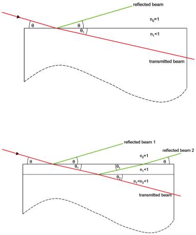
A monochromatic, well collimated beam impinges under a well defined, small angle αi = θ (in most cases θ 5o) onto the surface of the sample. It is then partly reflected specularly from the surface, i.e. the outgoing angle αf = θ as well, and partly refracted into the material (See Fig. 9.1). As we will derive below, the reflection from a laterally homogeneous medium can be treated according to classical optics. Only the proper index of refraction n has to be used.

For most material, the index of refraction for neutrons is slightly smaller than 1, leading to total external reflection for small angles of incidence θ < θc, where θc depends on the material.

In the case of a single layer on the substrate, reflection and refraction take place at both the surface and the interface (Fig. 9.2). Then, the reflected beams from the different interfaces interfere with each other. Maximum intensity is received, when the path length difference between the two reflected beams is an integer multiple of the wavelength.

For the case of perfectly smooth surface and interfaces, an exact description of the reflected and transmitted intensity can be deduced from quantum theory.

Fig. 9.1: Reflection and refraction from a free surface

Fig. 9.2: Reflection and refraction from a single layer on a substrate

9.2.1 Wave equation in homogeneous medium. Optical index

The starting point is the Schr¨odinger equation for the wave function of the neutron:

The kinetic energy of the neutron is given by E = 2k2/(2m) with the modulus k = 2π/λ of the wave vector k.

Due to the small |Q| values that are probed, a reflectometry experiment does not resolve the atomic structure of the sample in any of the three directions. Therefore, it is a valid approximation to describe the potential V1 of the homogeneous material as

where Nj is the number of nuclei per unit volume and bj is the coherent scattering length of nucleus j. With that we receive

with the wave vector k1 inside the medium. From this equation, it is justified to introduce the index of refraction in the material

positive for most isotopes), so that n is smaller than 1. This means that the transmitted beam is refracted towards the sample surface, which is opposite to the daily experience with light refracted at a glass or liquid surface.

9.2.2 Solution for a sharp surface. Fresnel’s formulas

In analogy to classical optics, we can derive e.g. Fresnel’s formulas. For the solution of the wave equation at a sharp surface between air and a semi-infinite medium, we assume the surface of the sample to be at z = 0. The potential is then

As the potential V is independent of the in-plane coordinates x and y, the wave function in the Schr¨odinger equation (9.4) is of the form

with the in plane components kx and ky of k independent of z. The Schr¨odinger equation then reduces to the one dimensional equation

where the index l distinguishes between vacuum (l=0) and medium (l=1). The unique solution is determined by the boundary conditions. The incoming wave in the vacuum before interaction with the sample is a plane wave of norm 1, i.e. t0 is equal to 1. In a half-infinite medium, there is no reflected wave, because there is nothing to reflect from, i.e. r1 vanishes. In addition, the wave function and its first derivative must be continuous at the interface. So we receive the following boundary conditions:

When we insert (9.9) into (9.10) we receive the continuity equations for the wave function:

t1 is the amplitude of the transmitted wave and r0 is the amplitude of the reflected wave. The reflectivity R is defined as the modulus squared of the ratio of the amplitudes or reflected and incoming waves, the transmissivity T is defined as the modulus squared of the ratio of the amplitudes or transmitted and incoming waves.

In conclusion, we arrive at the Fresnel’s formulas for the reflection and the refraction at a flat interface

9.2.3 Snell’s law of refraction. Total external reflection

Taking into account the continuity relation for the wave vector component tangential to the surface

together with k1 = k0n1 (Eq. 9.5), Snell’s law for refraction follows from trigonometry:

The fact that in most cases the index of refraction is n1 < 1 means that the transmitted beam is refracted towards the sample surface (θ1 < θ in Fig. 9.1). For angles of incidence θ below the so called critical angle θc with

total reflection is observed, i.e. all intensity is reflected and no wave propagating in z-direction exists in the sample. Only an evanescent wave in the z-direction with propagation parallel to the surface is induced. For angle of incidence above θc, the beam can partially penetrate the sample and is only partly reflected.

From Snell’s law (Eq. 9.17) and the definition of the index of refraction in Eq. (9.4) one can relate the normal components of the incoming and refracted wave vectors

This confirms that, for angles of incidence θ below θc, kz1 becomes purely imaginary and the refracted wave is an evanescent wave in the z-direction.

The last relation allows to express the Fresnel coefficients (Eq. 9.13 and 9.14) as a function of one variable only. In general the measured reflectivity is represented as a function of θ or the magnitude of the scattering wave vector Q = 2kz0:

When Q Qc, the preceding equation reduces to:

1 Q4

R c (9.20)

16 Q4

which is the formula for the reflectivity within the Born approximation [3]. This shows that the reflectivity above the critical angle decreases sharply with Q.

Once again, coming back to the wave function inside the surface, one finds using Eq. (9.18) that, when θ < θc:

This result is very important, because it shows that when the energy of the particle normal to

the surface is smaller than the potential barrier, the wave still can penetrate the medium on a

characteristic depth of 2/ Q2c − Q2. This evanescent wave propagates itself along the surface

with a wave vector equal to (kx, ky) and then leaves the volume in the specular direction. For example for Ni (ρ = 9.41×10−6 A˚ −2), the penetration depth is of the order of 200 A˚ at Q = 0; if one neglects absorption, it raises rapidly to infinity at Q = Qc. No conservation rule is broken: the reflectivity equals 1 because this wave represent no transmitted flux in the medium.

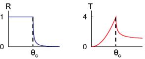
Fig. 9.3 represents, on a linear scale, the reflectivity and the transmissivity of a substrate as a function of the angle of incidence θ. The reflectivity equals 1 for angles smaller than the critical angle θc and decreases rapidly above this value (Eq. 9.20). The transmissivity increases monotonously up to a value of 4 at θc and decreases to 1 at large angles. This result might look very surprising at first sight. The value of 4 for the transmissivity comes from the fact that the incident and the reflected waves in vacuum superpose to form a stationary wave of amplitude exactly equal to 2 at the interface with the medium. For the intensity, we obtain a factor of 4.

Fig. 9.3: Reflectivity and transmissivity of a substrate as a function of the angle of incidence

9.2.4 Reflectivity from layered systems

In a layered system, the same Ansatz as in Eq. (9.9) can be written in each layer l. The coefficients of reflection rl and transmission tl can be deduced recursively from the continuity relations of the wave function and its derivative at each interface. If N is the number of layers, and considering the vacuum on top of the multilayer and the substrate below, 2(N+2) coefficients have to be calculated. The number of interfaces being N+1, the continuity relations lead to 2(N+1) equations. Two other equations are obtained considering that the transmission into the vacuum is equal to one (t0 = 1) and that, in the substrate, there is no reflected wave (rN+1 = 0), leading in total to a number of equations equal to the number of coefficients to determine. The calculation of the coefficients of reflection and transmission in each layer and, in particular, the calculation of the reflectivity in air are therefore possible [4].

Here we just want to demonstrate with very simple arguments how interference effects from layered structures arise and how the intensity modulations in Q-space are related to real space length scales.

Fig. (9.2) shows how interference can occur in a system composed of a single layer of thickness d deposited on a substrate. Interference occurs between beams reflected from the surface and those first transmitted in the layer, reflected from the interface between layer and substrate and then leaving the layer into vacuum. To a good approximation, refraction at the top surface can be neglected for incident angles twice the critical angle or total reflection. In this case θ = θ1 in Fig. (9.2) holds. Since the index of refraction of the neutrons is very close to one, this

approximation is valid even for rather small angles of incidence. Then the optical path length difference between the two beams is:

We can now determine the distance between interference maxima from the condition that the path length difference has to differ by one wavelength: λ = 2d · δ(sin θ) 2d · δθ. With Q = 4λπ sin θ 4λπ θ we final obtain:

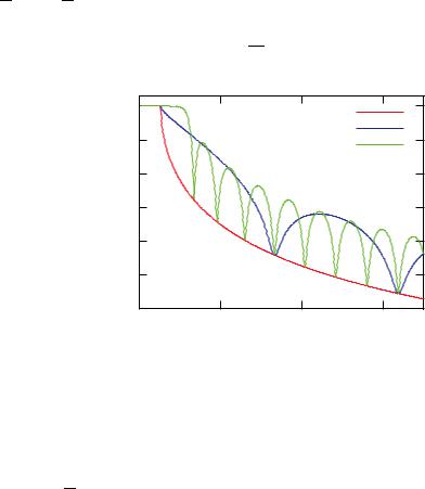
Fig. 9.4: Reflectivity of a Si substrate and reflectivity of a Ni layer (ρ = 9.41 × 10−6 A˚ −2) on Si substrate (ρ = 2.15 × 10−6 A˚ −2). Simulations are performed for two layer thicknesses d.

We can see that the interference phenomena in Q-space are connected with real space length scales in a reciprocal way. (9.23) tells us that there will be a number of interference maxima at a distance in Q of 2dπ . These interference phenomena are called “Kiessig fringes”. Fig. 9.4 shows calculations of the reflectivity of a Ni layer deposited on a Si substrate. One observes that the reflectivities above the critical angle for total reflection decrease rapidly, therefore the ordinate is on a logarithmic scale. The oscillations of the reflectivity due to the above described interference effect can be observed. At small angles, due to the effect of refraction, the interference maxima are a bit denser distributed than at higher angles where formula (9.23) can be used to determine the layer thickness from the distance between the interference maxima. The thinner layer corresponds to an interference scheme with a bigger period. In both cases the minima of the interference scheme lay on the reflectivity of the Si substrate.

Note that for a 100 A˚ thick layer of Ni, that has a scattering length density (SLD) approximately 4 times larger than the one of Si, the critical angle of total reflection is determined by the SLD

of Si and not by the one of Ni. This comes from the penetration depth of the neutrons that is bigger than 100 A˚ . For a 400 A˚ thick Ni layer, the θc approaches the one of Ni and the total reflection plateau is somewhat rounded.

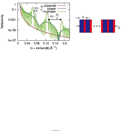
Fig. 9.5 shows the simulation of the neutron reflectivity from a multilayer on a Si substrate. This multilayer is composed of 10 double layers of 70 A˚ Ni and 30 A˚ Ti. On can clearly see the pronounced maxima due to the periodicity of the Ni/Ti double layer of thickness 100 A˚ . In between, one observes many weaker oscillation (be attentive to the logarithmic scale) with a period given by the total thickness of the multilayer.

Fig. 9.5: Reflectivities of a Ni/Ti bilayer and of a Ni/Ti multilayer on Si substrate. Simulations are performed for Ni and Ti thicknesses of 70 and 30 A˚ respectively.

9.2.5 Roughness and interdiffusion

Until now we assumed perfectly flat interfaces. A real interface will, however, always show a certain roughness at the atomic level, as shown in Fig. 9.6. The height profile of the interface is completely described by the parametrization z(x, y). Such a detailed information is not at all interesting. Much more interesting are parameters that statistically describe the interface, such as the mean squared deviation from an ideally flat interface, or the lateral correlation length. Those parameters can be determined from reflectometry and scattering under grazing incidence [5].

As simplest model, we assume that the height coordinate z follows a random distribution of values around the nominal value zj of the flat interface. The random distribution being described by a Gaussian function

the profile of index of refraction between layers j and j + 1 takes the form: