

76 |
C. Preibisch et al. |
|
|
•Perfusion parameters rCBV, CBF, and Ktrans—and their combinations—are good predictors of tumor grade (especially low-grade vs. high-grade) and outcome.
•Diagnostic accuracy is essentially augmented by perfusion data.
•Perfusion data combined with other metabolic imaging modalities helps in detection of pseudoprogression and pseudoresponse of gliomas.
2\ Methods
The delivery of oxygen and nutrients to cells via arterial blood through capillaries in biological tissue is referred to as perfusion. Blood flow—commonly used as a synonym of perfusion—denotes the rate of delivery of arterial blood to the capillary bed.
In a neuroradiological context, several surrogate markers have been derived to characterize tissue perfusion. The basic principle behind the measurement of perfusion-related parameters is the application of a tracer to the bloodstream, the distribution of which is then observed in the tissue. Since Stewart’s pioneering experiments, dating 1894 (Stewart 1894), a variety of approaches have been developed. Appropriately sized microspheres being trapped in tissue have for a long time been considered to be the gold standard in perfusion imaging, at least in animal studies (Bassingthwaighte et al. 1990; Heymann et al. 1977). More recently, freely diffusible tracers and positron emission tomography (PET) made perfusion measurement sufficiently noninvasive to allow an application in patients (TerPogossian and Herscovitch 1985; Raichle et al. 1983; Frackowiak et al. 1980).
The first magnetic resonance imaging (MRI)-based concepts of perfusion imaging emerged more than 20 years ago (Le Bihan 1992; Rosen et al. 1990; Villringer et al. 1988; Tofts and Kermode 1991) and have ever since been the subject of intense basic and clinical research. Because it yields valuable insights into tumor physiology and is widely available, MR perfusion imaging plays an important role in tumor differential diagnosis and grading as well as in therapy monitoring and follow-up (Faehndrich et al. 2011; Fatterpekar et al. 2012; Hattingen et al. 2008; Larsen et al. 2013; Mills et al. 2012; Wagner et al. 2011; Blasel et al. 2010).
In this section, we outline the principles of MR-based perfusion imaging with respect to different contrast mechanisms based on the manipulation of the longitudinal (T1) and transverse relaxation times (T2, T2*) as well as the implications of exogenous and endogenous contrast agent. Based on theoretical models that link MRI parameters with physiology, several surrogate markers of tissue perfusion can be deducted. In the first line, these are the cerebral blood flow
(CBF) denoting the rate of delivery of arterial blood to the tissue (commonly measured in [mL/100 mL/min]), the cerebral blood volume (CBV), i.e., the volume fraction of tissue occupied by blood vessels (commonly measured in [mL/100 mL] or [%]) and the mean transit time (MTT = CBV/ CBF). Useful phenomenological parameters are the bolus arrival time (BAT), time to peak (TTP), and relative MTT (rMTT, i.e., the full width at half maximum of the tissue concentration time curve). Furthermore, it is possible to determine a number of other markers characterizing vascular permeability and morphology like the volume transfer coefficient Ktrans and the vessel size index (VSI).
2.1\ Exogenous Tracer Methods
The most widespread methods for MR perfusion imaging rely on exogenous tracers, and the most common, clinically used contrast agents are chelates of paramagnetic gadolinium (Caravan et al. 1999), e.g., Gadolinium diethylene- triamine-pentacetate (Gd-DTPA). These extracellular fluid agents are considered as intravascular agents within the brain—as long as the blood–brain barrier is intact.
MRI contrast agents generally induce a shortening of MR relaxation times (i.e., an increase in corresponding relaxation rates). For longitudinal T1 relaxation, this is induced by a dipolar interaction between nuclear proton spins and unpaired electrons of the paramagnetic contrast agent (Caravan et al. 1999; Hendrick and Haacke 1993) which produces a signal increase in T1 weighted images. In areas with a disrupted blood–brain barrier, T1-based methods also allow estimation of vascular permeability (Tofts and Kermode 1991). On the other hand, the compartmentalization of a high magnetic susceptibility contrast agent within blood vessels produces long-range microscopic susceptibility gradients around the vessels, which accelerate transverse relaxation and thus effect a signal decrease in T2 or T2* weighted images (Villringer et al. 1988). The respective signal changes are measured via different imaging approaches, and perfusion-related parameters are deducted via appropriate physiological models. In principle, it is possible to measure CBV by obtaining measurements in the steady state before and after the application of an intravascular contrast agent with either T2* (Varallyay et al. 2013) or T1 weighted images (Lu et al. 2005; Wirestam et al. 2007). However, the most common methods applied in modern brain tumor perfusion imaging rely on dynamic imaging, which are described in the following sections.
2.1.1\ Dynamic Susceptibility Contrast MRI
In this most commonly applied method for perfusion imaging, the passage of a bolus of contrast agent is observed via T2* weighted imaging, and perfusion parameters are
MR Perfusion Imaging |
77 |
|
|
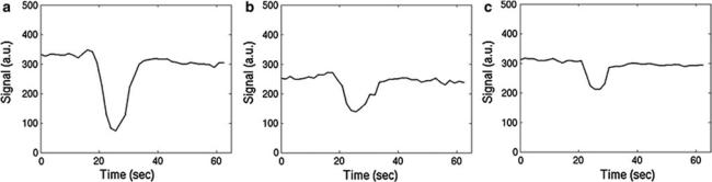
Fig. 1 Exemplary DSC signal–time curves obtained in arterial vessels (a), gray matter (b), and white matter (c)
derived by means of tracer dilution theories. First experiments were presented by Villringer et al. (1988). An introduction to the basic principles of tracer kinetic models as well as their application to bolus tracking MRI is given by Buxton (2009a), and a number of reviews cover all possible aspects of dynamic susceptibility contrast perfusion imaging (Le Bihan 1992; Calamante et al. 2002; Ostergaard 2004, 2005; McGehee et al. 2012).
In practice, a short bolus of contrast agent is injected into a peripheral vein and the subsequent signal changes occurring in the brain are monitored via T2* weighted imaging. Since the transit time of an intravascular agent is rather short (i.e., a few seconds), fast imaging methods are necessary to obtain a sufficient temporal resolution. Hence, echo planar imaging (EPI) (Turner et al. 1991), often in combination with parallel imaging (Deshmane et al. 2012), is commonly used as it allows to cover large portions of the brain with a reasonable temporal resolution of about 1 s. While T2* weighted gradient echo EPI is the most common method, T2 weighted spin echo EPI can also be used (Speck et al. 2000). Figure 1 shows characteristic signal–time curves obtained with T2* weighted dynamic susceptibility contrast (DSC) imaging.
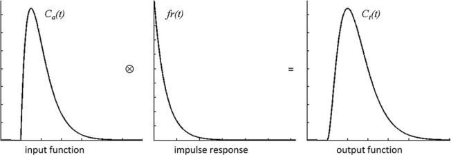
The challenge is now to transform the measured signal changes into valid measures of perfusion. Kinetic models relate the tracer concentrations in arterial blood Ca(t) and tissue Ct(t) to CBF, CBV, and MTT (Buxton 2009a). For an arbitrary arterial concentration–time course Ca(t) (arterial input function, AIF), the tissue concentration–time course Ct(t) (output function) depends on the local cerebral blood flow (CBF) as follows:
|
|
( |
) |
|
( |
) |
|
( ) |
\ |
|
\ |
Ct |
t |
|
= Ca |
t |
|
CBF r |
t |
|
(1) |
|
|
|
|
|
|
|
|
|
|
where r(t) is the local residue function and indicates convolution. The r(t) can be considered as the fraction of contrast agent molecules entering the tissue at time t = 0 and still being present at a time t > 0. Thus, the residue function is a monotonically decreasing function with r(t = 0) = 1; it contains the complexities concerning
details of contrast agent distribution and kinetics. For a single well-mixed compartment, r(t) is usually assumed to decay exponentially. The product CBF r(t) is also denoted as impulse response. Figure 2 illustrates the result of the convolution of idealized representations of an arterial con- centration–time curve and an impulse response to yield an idealized tissue concentration–time curve.
Based on Eq. (1) it can be shown that the peak of the impulse response is determined by CBF, while the area under the impulse response corresponds to the partition coefficient λ, which for common MR contrast agents can be considered as the distribution volume of the tracer, corresponding to CBV for intravascular agents (Buxton 2009a). According to the central volume theorem, the mean transit time MTT is given by CBV/CBF (Meier and Zierler 1954).
Using dynamic susceptibility contrast, it is relatively straightforward to calculate a relative CBV (rCBV) from the area under the measured signal–time curve. Because it is quite insensitive to the actual shape of the AIF, this quantity is considered to be a quite robust measure of rCBV as long as the relation between tissue concentration and signal intensity is the same throughout the brain (Buxton 2009a; Calamante et al. 2000). rCBV values are frequently normalized to healthy-appearing white matter to facilitate comparison between patients. Cerebral blood flow is much more difficult to obtain since for intravascular tracers the transit time is very short and thus the influence of CBF on the tissue concentration–time curve is rather subtle. Therefore, the bolus arrival time (BAT), the time to peak (TTP), and the relative mean transit time (rMTT), i.e., the full width at half maximum of the signal–time curve, are frequently used as surrogate markers of perfusion (Ostergaard 2004).
In order to obtain quantitative perfusion parameters from bolus tracking data, a deconvolution of the tissue concentra- tion–time curve Ct(t) with the arterial concentration–time curve Ca(t) (arterial input function, AIF) needs to be performed. However, unlike PET—where tracer concentrations are measurable quantities—the MR signal is only indirectly related to the contrast agent concentration. Usually, it is
78 |
C. Preibisch et al. |
|
|
Fig. 2 Relation of idealized concentration–time curves and impulse response according to Eq. (1)
assumed that the change in the transverse relaxation rate R2* is linearly related to the tissue concentration of contrast
agent (Rosen et al. 1990; Hendrick and Haacke 1993):
|
|
= k . C(t) \ |
(2) |
|
\ |
R2 |
|||
|
with a proportionality constant k. There are strong indications that this assumption of a linear relationship between the transverse relaxation rate and the concentration of the contrast agent is too simple (Blockley et al. 2008), because the mechanisms of signal loss in magnetically inhomogeneous media are highly complex (Blockley et al. 2008; Kjolby et al. 2006) and also depend on the vascular architecture (Johnson et al. 2000). Differential T2 and T2* relaxation behavior even allows to derive information on vessel diameter, size, and density (Kiselev 2005; Kiselev et al. 2005; Lemasson et al. 2013; Boxerman et al. 1995). Moreover, the contrast mechanisms within blood vessels and tissue are different (Kiselev 2001), and water exchange between tissue compartments actually needs to be taken into account (Landis et al. 2000; Li et al. 2010; Yankeelov et al. 2003). Nevertheless, Eq. (2) is usually employed to calculate tissue and arterial concentration–time curves from the measured MR signal with the echo time TE:
\ |
S (t ) = S0e−TEΔR2* (t) |
\ |
(3) |
|
|
|
For an absolute quantification of CBV, CBF, and MTT, the arterial input function, i.e., the arterial concentration– time curve Ca(t), needs to be measured with high accuracy, and in this respect, several additional difficulties occur. Usually, the AIF is measured in large arterial vessels crossing the imaging plane. However, because of the need for a high imaging speed, the spatial resolution is usually not sufficient to obtain pure blood voxels. This implies that partial volume effects most likely confound arterial signal
intensity. At high arterial contrast concentrations, a complete signal loss may occur inside large arterial vessels especially if EPI with long TE is used for data acquisition, which additionally distorts the AIF. While the AIF merely serves as a global scaling factor for CBV quantification, estimates of the local AIF would actually be required for valid measurement of CBF. This is related to the observation that any broadening and delay in the arterial input confounds the measured CBF (Calamante 2005; Calamante et al. 2004; Duhamel et al. 2006; Ko et al. 2007). Even with an appropriate AIF, valid CBF measurement with DSC remains a challenge. Given the fact that the influence of CBF on the measured tissue concentration–time curve is rather weak, the deconvolution process is very delicate and sensitive to noise (Ostergaard 2004, 2005; Ostergaard et al. 1996a, b). Hence, absolute quantification of perfusion parameters is rarely performed in clinical practice; instead, relative perfusion measures are normalized to healthy appearing WM or contralateral tissue. Therefore, valid comparisons for multicenter or longitudinal studies are hardly possible.
Additional difficulties arise from recirculation and extravasation of contrast agent to the tissue. While recirculation may cause a second broader and smaller peak about 30–60 s after the first pass of the bolus, extravasation prevents the signal from returning to baseline values. Therefore, a gamma-variate function is frequently fitted to the initial part of the signal–time curve (Belliveau et al. 1991; Boxerman et al. 1997) to remove the influence of recirculation and increase the reliability of CBV measurement. However, contrast agent extravasation, as in tumor areas with disrupted blood–brain barrier, causes more severe problems. Gd-DTPA outside the vasculature enhances T1 relaxation of tissue water, counteracting the susceptibilityinduced signal loss in T2* weighted images, which may lead to an underestimation of CBV (Rosen et al. 1990; Knopp et al. 1999; Quarles et al. 2009; Uematsu and Maeda
MR Perfusion Imaging |
79 |
|
|
2006; Essig et al. 2002). However, if the contrast agent outside the vasculature causes significant susceptibility gradients, an overestimation of CBV is likewise possible (Bjornerud et al. 2011). There are several methods to account for contrast agent leakage in DSC-based CBV measurement. One practical possibility to reduce the influence of T1 relaxation is the administration of a pre-bolus of contrast agent in order to saturate the tissue in the leakage area (Paulson and Schmainda 2008; Boxerman et al. 2012). More elaborate approaches comprise double echo acquisitions (Uematsu and Maeda 2006; Paulson and Schmainda 2008; Miyati et al. 1997; Heiland et al. 1999; Vonken et al. 2000) or sophisticated data analysis (Rosen et al. 1990; Quarles et al. 2005, 2009; Bjornerud et al. 2011; Uematsu et al. 2000; Johnson et al. 2004), which also provides information on vessel permeability and seems to reveal a benefit when compared to the application of a pre-bolus alone (Boxerman et al. 2012). Valid quantification of perfusion using DSC, especially in areas with contrast agent leakage, is a matter of intense research. Since the blood–brain barrier in tumors is frequently disrupted, new developments would be highly relevant.
In spite of these issues, DSC-MRI is by far the most frequently used perfusion imaging method, as it is easy to perform and yields robust information on tissue perfusion, i.e., rCBV.
2.1.2\ Dynamic Contrast-Enhanced MRI
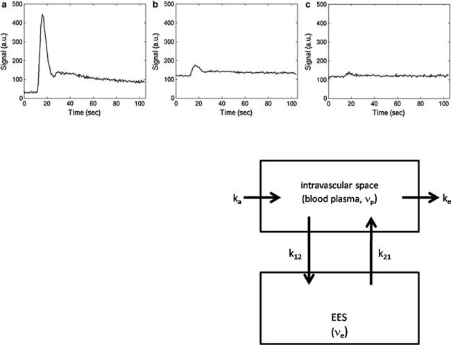
A qualitatively similar approach to perfusion imaging relies on the acquisition of a time series of T1 weighted images during bolus application (Fig. 3). This method is termed dynamic contrast-enhanced (DCE) imaging and allows quantification of vessel permeability, which is merely a confounding factor in DSC-based perfusion imaging. Generally, DCE-MRI requires the acquisition of a time series of T1 weighted images over several minutes to observe the wash-in and washout of contrast agent in extravascular extracellular space. Qualitative or semiquantitative measurements of leakage-related parameters are relatively easy to perform. The slope of the wash-in and washout portions of the time course can be evaluated within the regions of interest, allowing the distinction of tumor (fast rise) and radiation necrosis (slow rise) (McGehee et al. 2012). Also, semiquantitative parametric maps of the wash-in and washout slopes, maximal enhancement, and arrival time can easily be created. Integration of the initial area under the DCE tissue concentration curve (initial AUC) yields a more quantitative parameter (Li et al. 2012; Sourbron et al. 2009; Sourbron 2010) without the need for a sophisticated model. However, the influence of underlying physiologic processes like vessel permeability, extravascular extracellular volume, and blood flow is rather unclear (Donahue et al. 1996).
Similar to the DSC method, quantitative DCE-based perfusion measurements are quite elaborate (Yankeelov and Gore 2009; Sourbron and Buckley 2012, 2013). Quantitative approaches require complex pharmacokinetic models, a quantitative relation between MR signal and contrast agent concentration, as well as an appropriate AIF. Pharmacokinetic models describe the distribution and elimination of contrast agents within and from the tissue with respect to the underlying physiology. Most frequently, a two-compartment model is used based on the pioneering work of Kety (1951). This model describes the tissue as consisting of an intravascular space (plasma volume vp) and an extravascular extracellular space (EES, volume ve) (Fig. 4). The distribution of the contrast agent is characterized by arterial delivery and venous elimination rates ka and ke as well as distribution and redistribution rate constants k12 and k21, which describe the diffusion into EES. Commonly measured parameters are the volume transfer constant Ktrans between blood plasma and EES
\ |
K trans = E CBF (1− Hct) \ |
(4) |
|
|
(with extraction fraction E and hematocrit Hct), the EES volume fraction ve, and the rate constant between EES and blood plasma kep = Ktrans/ve. However, the interpretation of Ktrans depends on the physiological conditions: when the vessel permeability is much higher than blood flow (flow-limited condition), Ktrans corresponds to the blood plasma flow per unit volume of tissue; when blood flow is much higher than vessel permeability (permeability-limited condition), Ktrans corresponds to the permeability surface area product per unit volume of tissue (Sourbron and Buckley 2011).
First quantitative approaches were hampered by a rather low temporal resolution of T1 weighted imaging data and therefore only allowed to obtain Ktrans and ve as primary parameters for tissue characterization (Tofts and Kermode 1991; Tofts 1997; Tofts et al. 1999; Larsson et al. 1990; Brix et al. 1991). As technical progress permitted T1 weighted imaging with sufficiently high temporal resolution, advanced models have been developed which additionally allow measurement of CBV and CBF (Sourbron and Buckley 2012; Henderson et al. 2000; Pradel et al. 2003; Brix et al. 2004; Larsson et al. 2009; Li et al. 2012; Sourbron et al. 2009). Comprehensive reviews on these methods are given by Yankeelov and Gore (2009) as well as Sourbron and Buckley (2012, 2013), Sourbron (2010).
The majority of DCE-based MRI experiments are based on a model originally developed by Tofts (Tofts and Kermode 1991). According to that, the intravascular signal contribution is neglected and the relation between the contrast agent concentrations in tissue Ct(t) and blood
80 |
C. Preibisch et al. |
|
|
Fig. 3 Typical DCE signal–time curves obtained in arterial vessels (a), gray matter (b), and white matter (c)
plasma Cp(t) is described by (Yankeelov and Gore 2009; Tofts et al. 1999)
|
∫ |
K trans |
( |
t − t′ |
) |
|
|
|
|
|
|
|
|
||||
Ct (t ) = K trans |
|
Cp (t ) exp |
|
ve |
|
dt ’. |
(5) |
|
\ |
|
|
|
|
\ |
|||
|
|
|
|
|
|
|
|
|
Inclusion of a plasma compartment with a volume vp yields the extended Tofts model (Sourbron and Buckley 2012; Brix et al. 2004):
|
|
|
K trans |
( |
t − t′ |
) |
|
|
Ct (t ) = vp Cp(t ) + K trans |
∫ |
Cp (t ) exp |
|
|
dt ’. |
|
||
|
|
|
|
|
||||
|
|
|
ve |
|
|
\ |
||
\ |
|
|
|
|
|
|||
|
|
|
|
|
|
|
|
|
|
|
|
|
|
|
|
|
(6) |
Estimates of perfusion parameters are usually obtained by multiparametric nonlinear fitting of these equations to measured concentration–time curves. Besides that, a large number of different approaches have been developed. A recent comprehensive review of a variety of currently existing models for DCE-based perfusion measurement is given in Sourbron and Buckley (2013).
Similar to the DSC method, the measured T1 weighted MRI signal needs to be converted to contrast agent concentration before quantitative evaluations can be performed. Usually, a linear relation between the change in the longitudinal relaxation rate R1 (= 1/T1) and contrast agent concentration is
assumed (Landis et al. 2000; Yankeelov and Gore 2009): |
|
|
\ |
R1 (t ) = r1 C (t ) + R10 \ |
(7) |
|
|
|
with the contrast agent relaxivity r1 and the precontrast relaxation rate R10. This assumption regards biological tissue as a single well-mixed compartment or at least requires a fast exchange of water between all tissue compartments. However, there are indications that water exchange is not fast enough in the presence of contrast agent (Donahue et al. 1996; Parkes and Tofts 2002; Schwarzbauer et al. 1997). Accounting for the water exchange rates between different tissue compartments even allows determination of
Fig. 4 Two-compartment model: Contrast agent is delivered to the intravascular space with a rate constant ka and is eliminated with a rate constant ke. The CA diffuses into and outside of the extravascular extracellular (EES) space with a distribution rate constant k12 and a redistribution rate constant k21
intravascular or extravascular intracellular lifetimes of water molecules (Yankeelov and Gore 2009). Since a high temporal resolution is needed, R1(t) cannot be measured directly. Instead, R1(t) is determined from the T1 weighted signal–time curve s(t) and a precontrast measurement of tissue R10 where the exact formula depends on the imaging sequence. For a saturation recovery sequence with time delay TD, the tissue concentration curve is calculated according to
|
|
|
1 |
|
|
s |
t |
) |
|
|
R10 |
|
|
|
C (t ) = − |
|
ln 1 |
− |
|
( |
|
− |
|
(8) |
|||
|
r1 |
TD |
|
s0 |
|
r1 \ |
|||||||
\ |
|
|
|
|
|
|
|
|
|||||
|
|
|
|
|
|
|
|
|
|
|
|
|
|
Precontrast T1 mapping is frequently performed using the variable flip angle approach because it allows fast imaging with whole brain coverage (Yankeelov and Gore 2009; Li et al. 2012; Roberts et al. 2006; Harrer et al. 2004).
MR Perfusion Imaging |
81 |
|
|
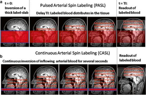
Fig. 5 Schematic order of events for pulsed (a) and continuous (b) arterial spin labeling (ASL)
However, this method needs careful spoiling or correction for the influence of residual magnetization to be accurate. At field strengths of 3 T and above, additional mapping of the local flip angle is required (Preibisch and Deichmann 2009). Therefore, saturation or inversion recovery methods are also frequently used (Larsson et al. 2008; Deichmann 2005; Henderson et al. 1999; Zhu and Penn 2005).
Also, a valid AIF, i.e., the plasma concentration of contrast agent Cp(t), needs to be determined for quantitative perfusion measurements. In this respect, similar limitations as in DSC imaging apply, e.g., with respect to partial volume effects, broadening, and delays (Yankeelov and Gore 2009). However, unlike in DSC imaging, the linearity of signal change inside vessels is of less concern since there is no complication due to complete signal loss at high contrast agent concentrations.
The major drawback of DCE-MRI in comparison to DSC- based perfusion imaging is the significantly reduced signal change, which results in rather low SNR in the calculated parameter maps. In practice, it is also much more demanding to achieve a reasonable spatial coverage and temporal resolution with T1 weighted imaging methods, and it is more difficult to choose an appropriate method from the large variety of different approaches (see Sourbron and Buckley 2013 for a recent review).
2.2\ Endogenous Tracer Methods: Arterial
Spin Labeling
Arterial spin labeling is an alternative agglomeration of methods for measurement of cerebral blood flow which uses magnetically labeled water in blood vessels as endogenous diffusible tracer. The basic idea is to acquire two data sets,
one with labeling of inflowing blood and one without. The difference signal is proportional to the delivered magnetization and hence to blood flow. Because labeled water acts as a freely diffusible tracer with accordingly prolonged tissue transit times, CBF derived from arterial spin labeling (ASL) is principally more robust than CBF derived from bolus tracking based on intravascular tracers (Buxton 2009b). Figure 5 depicts the basic order of events for the two fundamental types of pulsed (PASL) and continuous arterial spin labeling (CASL).
In the PASL labeling condition, a thick slab proximal to the imaging volume of interest (blue framed slab in (a)) is usually inverted at time t = 0 by a short RF pulse. After a delay time (inversion time, T1, typically ≈1.5 s), which allows labeled blood to distribute within the imaging volume, labeled images are acquired. CASL approaches use extended labeling periods where inflowing blood is inverted continuously by long RF pulses (several seconds) in a thin slice in the neck area. Labeled images are acquired after termination of the labeling pulse. A recent development is the pseudocontinuous ASL (pCASL) approach, where series of short RF and gradient pulses achieve more efficient labeling (compared to PASL) and reduced specific absorption rate (SAR) and magnetization transfer effects (compared to CASL) (Silva and Kim 1999; Wu et al. 2007; Helle et al. 2012). Remarkably, it is also possible to selectively label individual arterial vessels, which enables imaging of vascular territories (Helle et al. 2012; Golay et al. 2005; Paiva et al. 2007; van Laar et al. 2008).
Qualitative perfusion images can easily be derived because the difference between labeled and unlabeled images is proportional to CBF, but absolute quantification is again quite difficult. A good introduction to ASL is given by Buxton (2009b) and a number of recent reviews cover
82 |
C. Preibisch et al. |
|
|
all possible methodological issues (Wu et al. 2010; Deibler et al. 2008; Golay and Petersen 2006; Golay et al. 2004; Williams 2006; Parkes 2005; Petersen et al. 2006a, b) with regard to ASL-based CBF quantification.
Generally, care needs to be taken with regard to the control experiments because the labeling pulse, though applied off resonance, may nevertheless affect the magnetization within the imaging volume mainly via magnetization transfer effects (McLaughlin et al. 1997; Pekar et al. 1996; Zhang et al. 1992). Since the signal change inferred by blood flow only is on the order of about 1 %, even small effects may introduce large errors. To control for magnetization transfer effects, an equivalent off-resonant RF pulse needs to be applied during the control condition without labeling the inflowing spins. A number of techniques have been developed for all types of ASL methods, even though the effect is much more severe in CASL due to the long duration of its labeling pulse (Buxton 2009b). PASL approaches mainly vary by different placement of the control RF pulse (Edelman et al. 1994; Kwong et al. 1995; Wong et al. 1997; Kim 1995), while some CASL techniques even use separate labeling coils in the neck (Shen and Duong 2011; Paiva et al. 2008; Talagala et al. 2004). In PASL, slice profile effects due to the close proximity of the labeling slab and the imaging slice are also a problem and are usually diminished by a gap between labeling and imaging slice. Because the ASL difference signal change is so small, suppression of the static tissue signal (background suppression) in the imaging slices was found to be beneficial (Garcia et al. 2005; Mani et al. 1997; Ye et al. 2000).
Major confounding factors are transit delays t between the labeling plane and the imaging slice (Zhang et al. 1992; Wong et al. 1997; Alsop and Detre 1996; Buxton et al. 1998), the bolus duration T (Buxton 2009b; Wong et al. 1998; Luh et al. 1999), and relaxation effects (Buxton 2009b). The transit delay t may vary across the brain by several tenth of milliseconds (Wong et al. 1997) causing systematic errors even in qualitative CBF maps. An effective means to reduce the influence of transit delays in CASL is to insert a delay after the end of the labeling pulse (Alsop and Detre 1996); for PASL, the inversion time needs to be longer than the longest t. In CASL, the duration of the arterial bolus is well defined by the duration of the labeling RF pulse. In PASL, however, the thickness of the labeling slab determines the amount of labeled blood, and the bolus duration thus depends on global flow (Buxton 2009b). In order to create a bolus with a well-defined duration, saturation pulses can be applied to the labeling slab after an inversion time TI1 (Wong et al. 1998; Luh et al. 1999). The most complex effect is caused by water exchange between vessels and tissue. Initially, when labeled water is delivered to the tissue, relaxation of water spins occurs within the vessels with the arterial longitudinal relaxation time T1A, while after exchange—within the brain parenchyma—the
tissue relaxation time T1t applies. This is difficult to model, especially since the exchange time Tex (on the order of a few tenth of seconds) is not well known (Buxton 2009b).
Quantitative evaluations need to account for these effects. Early approaches used a modified Bloch equation to account for the influence of CBF on the difference signal (Kwong et al. 1992, 1995; Kim 1995; Detre et al. 1992). More recently, tracer kinetic modeling has also been used to derive CBF from ASL data (Buxton et al. 1998). In this approach, the amount of magnetization delivered to the imaging voxel by arterial blood
M(t) (i.e., the magnetization difference between control and label condition) is regarded to correspond to the tracer concentration. Based on this presumption, tracer kinetic principles can be applied to describe the influence of physiological processes on M(t) by means of a delivery function c(t), a residue function r(t), and a magnetization relaxation function m(t) (Buxton 2009b; Buxton et al. 1998):
|
|
( |
) |
= 2M |
0 A |
( |
) |
( |
) |
( ) |
\ |
|
\ |
M |
t |
|
|
CBF c t |
|
r t |
|
m t |
|
(9) |
|
|
|
|
|
|
|
|
|
|
|
|
|
where denotes convolution. The equilibrium magnetization of arterial blood M0A is difficult to measure, but a useful approximation can be obtained from the CSF signal (Chalela et al. 2000). Appropriate definitions of the functions c(t), r(t), and m(t) allow to include the effects of transit delays t and delayed water exchange Tex (Buxton 2009b):
0
ae−t /T
c (t ) = 1A
ae−t /T1A0
r (t ) = e−CBF t /l
e−t /T
m(t ) = 1A
\
e−Tex /T1A
(PASL) (CASL)
e− (t −tex )/T1t
0 < t < |
t |
t < t < |
t + T |
t < t < |
t + T |
t < T < t |
|
|
(10) |
t > Tex |
|
t > Tex |
\ |
with bolus length T, inversion efficiency α (Alsop and Detre 1996; Zhang et al. 1993), and the longitudinal relaxation times of water in arterial blood and tissue T1A and T1t. Generally, absolute CBF quantification is quite laborious because several time points need to be acquired after the end of the labeling pulses for proper modeling in CASL as well as PASL (Petersen et al. 2006a, b, 2010). This is aggravated by the fact that the SNR of a single difference image is quite low meaning that several (≈50) averages need to be acquired. T1A of arterial blood is usually assumed from the literature, but mapping of local tissue T1 is considered to be necessary, especially with CASL because the longer labeling duration allows more time for exchange (Buxton 2009b; Parkes 2005). Reduced inversion efficiency is rather a problem in CASL (Alsop and Detre 1996; Zhang et al. 1993), while proper definition of bolus duration is a bigger issue in PASL (Wong et al. 1998; Luh et al. 1999). There are a number of