

10 |
1 Electromagnetic Field and Wave |
(a) |
(b) |
PORT INPUT |
PORT INPUT |
OUTPUT PORT |
OUTPUT PORT |
(c)
INPUT INPUT PORT PORT
OUTPUT OUTPUT
PORT PORT
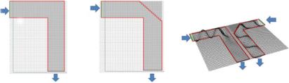
Fig. 1.4 Different transmission characteristics of the microwave transmission line under DC and time-varying conditions
Example 1.1 Connect a metal point to the “ground” with a metal wire; then, the potential of the metal point is the same as the “ground” potential. However, it should be noted that this conclusion can only be strictly established when the entire system is time invariant. In other words, when the frequency is high enough that the linearity (maximum length) of the metal wire can be compared with the wavelength, the phases of the entire metal wire will be unequal since the electrical size (ratio of the geometric size to the wavelength) of the metal wire is large. Therefore, the metal point is no longer equipotential to the “ground” potential.
Example 1.2 Figure 1.4 illustrates a microwave transmission line. The difference between Fig. 1.4a and b is their corners: Fig. 1.4a has a right angle and b has a chamfer angle.
There are input signals at the input port respectively. If the input is a DC signal, there is no difference in the output signal obtained at the output port. However, when the input signal is high frequency or even microwave signal, the situation changes qualitatively. For an easier comparison, the signal transmissions of Fig. 1.4a, b are put together as shown in Fig. 1.4c. It can be seen from this figure that when the corner is a right angle, the output port has no output signal, and a standing wave is formed on the input arm; in case of a chamfer at the corner, there is output signal at the output port.
1.2 Electromagnetic Power Flux
By learning the concept of microwave power flux, our readers can understand that: 1. Even in the case of DC, the energy transmitted by the voltage source to the electronic load can be transmitted through the free space; 2. the properties of devices like capacitors, inductors, and resisters are depend on its energy storage and energy consumption characteristics.

1.2 Electromagnetic Power Flux |
11 |
Electromagnetic field is a special form of material existence. Although the electromagnetic field has no static mass, it has the performance of energy and force. For example, solar energy is a kind of electromagnetic energy; the electrostatic force, the magnet’s attraction to the ferromagnetic field, and the magnetic force generated around the current indicate that the electromagnetic field has force.
In this section, we will first study the possible transmission channels of electromagnetic energy from the perspective of electromagnetic power influx to further explain the coupling channels in EMC research. Then, the relationship between the properties of the resistors, inductors, capacitors, and their internal electromagnetic fields is studied from the perspective of electromagnetic fields to reveal the nature of the components: Resistors are energy-consuming components, and inductors and capacitors are energy storage components. This research is especially important when a system cannot be described by lumped variables like resistance, inductance, and capacitance.
1.2.1 The Transmission of Electromagnetic Power Flux
In this section, we explain that the electromagnetic fields are capable to carry energy, and wherever there is a field, there is electromagnetic energy.
From the electromagnetic field theory, we see that the electric field energy density for the electrostatic field problem is:
wE 1/2ε0 E(r) · E(r) J /m3 |
(1.4) |
The total electric field energy distributed in space is:
WE |
1 |
V ε0 E(r) · E(r)d V ( J ) |
(1.5) |
2 |
The integration area covers the whole space.
For a constant magnetic field problem, the magnetic field energy density is:
wH (r) |
1 |
μ0 H(r) · H(r) J /m3 |
(1.6) |
2 |
By integrating the full space, we can get the total magnetic field energy distributed in the whole space
WH |
1 |
V H(r) · μ0 H(r)dV ( J ) |
(1.7) |
2 |
The definition of wE (r) and wH (r) are also applicable to the time-varying field, i.e.,

12 |
|
|
|
1 |
Electromagnetic Field and Wave |
|
wE (r, t) |
1 |
ε0 E(r, t) · E(r, t) |
J /m3 |
(1.8) |
||
|
|
|||||
2 |
||||||
wH (r, t) |
1 |
μ0 H(r, t) · H(r, t) |
J /m3 |
(1.9) |
||
|
||||||
2 |
||||||
The total energy density of electromagnetic field is |
|
|
||||
w(r, t) wE (r, t) + wH (r, t) |
J /m3 |
(1.10) |
||||
By integrating the full space, we can get the total electromagnetic field energy distributed in the whole space
W |
1 |
V (ε0 E(r, t) · E(r, t) + μ0 H(r, t) · H(r, t))d V |
(1.11) |
2 |
The analysis above shows that for static electric fields, electric field energy exists wherever E 0; for a constant magnetic field, the magnetic field energy exists wherever H 0; for electromagnetic waves, as long as the electromagnetic field is not equal to zero, electromagnetic energy exists.
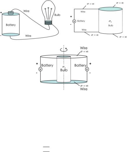
The fact that wherever there is electromagnetic field there is electromagnetic energy indicates that electromagnetic energy can be propagated in space. Here, we use the practical application of the flashlight to explain that even in the case of DC, the energy output from the DC voltage source can be transmitted to the resistor in space between the voltage source and the load. The circuit model of the flashlight is consisted of a DC voltage source, a wire and a resistance. To facilitate an accurate, we modified the model in premise of retaining the working principle.
Now, we take Fig. 1.5 as an example to analyze how the energy supplied from the DC voltage source (battery) is transferred to the load (bulb). Here, we use column
ˆ ˆ
coordinate system (the variables are rc, ϕ and z, and the unit vectors are irc , iϕ and
ˆz ). Then, we build a analysis model as shown in Fig. 1.5c. There is a linear, uniform, i
cylindrical resistor rod (with electric conductivity σ ,length d, and radius a). Its two ends are connected to two circular parallel plates with conductivity σ equals ∞,and radius b > a. At the position of rC b, the system is excited by a circularly symmetric voltage source and the potential difference between the plates is kept to be a constant V0.
This is a system unrelated to ϕ. The electric field between the plates is a uniform field, i.e.,
V0 |
|
|
E −iz d |
(V/m) |
(1.12) |
Under the excitation of an electric field, a current is generated in the resistance bar, and the current density is
1.2 Electromagnetic Power Flux |
13 |
(a) Flashlight; |
(b) working principle of a flashlight; |
|
(c) analysis model.
Fig. 1.5 Example of power flux analysis
J(r) σ E(r) −iz V0σ/d ( A/m2)
The total current in the rod is I0 S J(r) · da σ V0π a2/d ( A).
Using Ampere’s loop law, the magnetic field of the system can be determined as:
−i ϕ I0 rC2
2π a
H −i ϕ 2 I0r
π C
0
(0 ≤ rC < a, 0 < z < d) |
|
(a < rC < b, 0 < z < d) ( A/m) |
(1.13) |
(rC > b, 0 < z < d) |
|
Poynting vector is S(r) E(r) × H(r). It is not difficult to see that in the area of
0 ≤ rC < a, there is |
|
|
|
|
|
||
S(r) E(r) × H(r) −iz |
V0 |
× −iϕ |
I0rC |
−irC |
V0 I0 rC |
W/m2 |
|
d |
|
2π a2 |
2π d a2 |
||||
|
|
|
|
|
|
|
(1.14) |
In the area of a < rC < b, there is |
|
|
|
|
|
||
14 |
1 Electromagnetic Field and Wave |
Fig. 1.6 Distribution of
Poynting’s vector S(r)
S(r) E(r) × H(r) −iz |
V0 |
× −iϕ |
I0 |
−irC |
V0 I0 |
W/m2 |
d |
2π rC |
2π d rC |
||||
|
|
|
|
|
|
(1.15) |
Outside the system, i.e., in the area rC > b, since H(r) 0, there is S(r) 0. Using Poynting’s theorem, the distribution of electromagnetic power flux density
can be obtained as:
|
|
|
|
|
− |
V0 I0 |
−σ |
V02 |
≤ rC < a) |
|
|
1 ∂ |
|
|
|
(0 |
|||||
· S(r) |
|
π a2 d |
d2 |
|||||||
|
|
|
rC SrC |
|
|
|
|
|
W/m3 (1.16) |
|
rC |
∂rC |
|
|
|
|
|||||
|
|
|
|
|
0 |
|
|
|
(rC > a) |
|
It can be seen from formula (1.16), in the air domain of a < rC
no dispersion; that is, the field lines are continuous in this area. It indicates that only the electromagnetic power is transmitted in the air domain, and there is no loss of electromagnetic power.
However, inside the resistor rod, the divergence of S(r) is negative; thus, the field line should be terminated within the resistance bar, so the Poynting vector is absorbed inside the resistance bar, which indicates that there is a loss of electromagnetic power. It can be calculated that the electromagnetic power density of the loss in the resistance bar is
pd σ | E(r)|2 σ V02 d2 (W/m3)
Figure 1.6 is a schematic diagram of the distribution of the vector S(r). It can be clearly seen that the energy flux is transmitted from the DC voltage source to the loads through the space in between.
As it can be seen from Fig. 1.6, in an ideal conductor plate, there is no electromagnetic power flux and the flux only distributes in the air. It shows that the power applied to the resistor by the power supply does not flux through the conductor plate to the resistor, but is applied to the resistor through the air field around the resistor rod. This is different from the concept in circuit theory. According to the electromagnetic field theory, electromagnetic power is transmitted through space, and the conductor only serves to guide the electromagnetic field (i.e., boundary conditions).