6.3.3The Collaborative Optimization Method for Multiple EMC Indicators

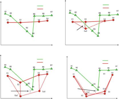
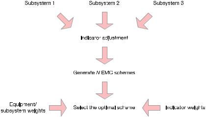
Fig. 6.15 Collaborative design method of indicator

indicator space to rank the schemes according to their advantages and disadvantages. The general steps for ranking the schemes using the TOPSIS method are as follows:

(1)Construct an initial evaluation matrix C.

(2)Normalize the decision matrix.

(3)Calculating a weight matrix for the normalized matrix in (1).

(4)Determine the positive ideal point X+ and the negative ideal point X−.

(5)Calculate the Euclidean distance of each scheme to the positive ideal point di+ and the negative ideal point di−.

(6)Calculate the closeness of each solution to the ideal solution di .

(7)Rank the schemes in descending order di .

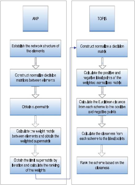
ANP-TOPSIS scheme evaluation (Fig. 6.16): First, identify the indicators to be involved in the evaluation and design; then construct the network (ANP) of the evaluation system, including the calculation of the unweighted supermatrix, the weighted supermatrix and the limit weighted supermatrix; finally, rank the schemes according to TOPSIS, including constructing the normalized decision supermatrix, determining the positive ideal point and the negative ideal point of the weighted normalization matrix, calculating the Euclidean distance from each scheme to the positive ideal point and the negative ideal points, calculating the closeness of each scheme to the ideal point, and ranking the schemes according to the closeness. The parameters in the ranked scheme are the parameters of the indicator decomposition, as shown in Fig. 6.16.

Since the aircraft EMC indicators appear in many types such as precise number, interval number, and fuzzy number [69], the evaluation of aircraft EMC is a multiattribute decision-making problem of indicators. For the convenience of our readers,

Fig. 6.16 Flowchart of scheme evaluation

288 6 Application Cases of System-Level EMC Quantitative …

where and represent the addition and multiplication of fuzzy numbers, respectively.

Now, we explain the ANP-TOPSIS method using the EMC design of the communication station as an example. The comprehensive evaluation indicators of the communication station are receiver sensitivity, IF rejection ratio, transmitter power, antenna isolation, VSWR of antenna, case shielding effectiveness, and frequency band coupling.

First, the weights of the indicators are calculated using ANP method, as shown in Table 6.7. Next, the seven design indicators are listed as a set Q {Q1, Q2, . . . , Q7} where in terms of indicator attributes, Q1 and Q3 are interval number indicators; Q2, Q4, Q5, and Q6 are precise number indicator; Q7 is the fuzzy indicator. Q6 is a score value, ranging from 1 point (worst) to 10 points (best). Q7 is a level indicator, which includes seven levels: “no coupling,” “not serious at all,” “not serious,” “common,” “serious,” “very serious,” and “extremely serious.” In terms of indicator types, Q1, Q2, Q4, and Q6 are indicators of benefit (the bigger the better), and the other three are indicators of cost (the smaller the better).

There are four shortwave radio design solutions, and we need to select a good one. These four schemes are defined by the metrics of the seven indicators. For example, in scheme 1, the short-wave receiver has a sensitivity range of 90–105 dBm in various adjustment modes and an IF rejection ratio of 65 dB. The short-wave transmitting power range is 60–85 W. The antenna isolation with a certain piece of core equipment is 55 dB. The VSWR of the antenna is 1.2. The shielding effectiveness of the case is 7 dB. The frequency band coupling with other frequency equipment of the whole aircraft is at a common level. The EMC indicators of these four design schemes are listed in Table 6.7.

Firstly, the fuzzy number of the indicator Q7 is analyzed and calculated. According to the corresponding relationship between the triangular fuzzy number and the

Table 6.7 EMC performance indicators of the four design schemes

language description variable introduced above, the qualitative indicator is represented by the triangular fuzzy number. The seven levels of the indicator, from low to high, are expressed as (0 0 0.1), (0.1 0.2 0.3), (0.2 0.3 0.4), (0.4 0.5 0.6), (0.6 0.7 0.8), (0.8 0.9 1.0), and (0.9 0.9 1.0). Then, we can derive the decision matrix

According to the above equations, the positive ideal point X+ and the negative ideal point X− are calculated as

X + [(0.1011, 0.1427), 0.0651, (0.0731, 0.1360), 0.1018, 0.1018, 0.0785, (0.0187, 0.0515, 0.1439)]

X − [(0.0859, 0.1189), 0.0576, (0.0621, 0.1020), 0.0746, 0.0679, 0.0491, (0.0053, 0.0111, 0.0240)]

The Euclidean distance di+ from each scheme to the positive ideal point X+\ and the distance from X− to the negative ideal point di− can be determined

Finally, the closeness of the four schemes to the positive ideal point is calculated

as

According to the above calculation results, the ranking of the advantages and disadvantages of the scheme can be obtained. For the design of a communication station, the comparison results of the four schemes given in Table 6.7 are scheme 1 > scheme 2 > scheme 3 > scheme 4.