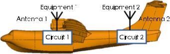
Fig. 6.6 Diagram of the equipment installation

PS AT PB + 10 lg( f / fO R )

where PA, PB, f fO R and (R) are the same as previously defined.

Since the level of the functional signal PD is usually unknown, it is considered that PD − PR E F is in a dynamic range, and the amount of desensitization calculated in this situation will be smaller. According to the desensitization curve shown in Fig. 6.5a, the slope R can be obtained using PD − PR E F ; according to the saturated reference power curve shown in Fig. 6.5b, the saturation reference power PB of the receiver can be calculated using PD − PR E F ; then, we can obtain the desensitization value.

6.2.2 Field–Circuit Collaborative Evaluation Technique

The electromagnetic field generated by external electromagnetic field, antenna radiation field, case and cable can be equivalent to sources at circuit level. Then, we can do comprehensive EMC simulation at circuit level. This technology is called field–circuit hybrid technology.

Aircraft platforms, airborne equipment, installed cables, and antennas form complex conduction or radiation coupling cross-linking relationships, resulting in complex field–circuit coupling relationships among aircraft equipment/subsystems. Therefore, it is necessary to carry out comprehensive simulation analysis of the system from the aspect of electromagnetic field and circuit; i.e., we need to perform corresponding electromagnetic simulation, and fully consider the influence of electromagnetic environment in equipment-level circuit simulation analysis.

Figure 6.6 shows the pair of transmitting/receiving equipment that are likely to interfere with each other in the interference pair decision. Both equipment 1 and equipment 2 are composed of an antenna and a circuit, respectively. When analyzing the mutual interference situation of this transmitting–receiving equipment pair, it is necessary to separately model and simulate the antenna and circuit of the two equipment, and equivalent the field simulation result into a circuit module, which is later imported into the circuit for synthesis simulation.

(a)

(b)

(c)

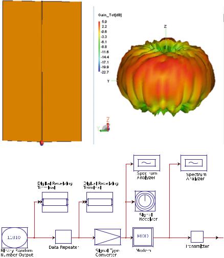
Fig. 6.7 Equivalent model of equipment 1, a antenna model; b antenna pattern; c circuit model

The antenna of equipment 1 is modeled as shown in Fig. 6.7a. The threedimensional far-field characteristics of antenna 1 are shown in Fig. 6.7b. The circuit of equipment 1 is modeled as shown in Fig. 6.7c.

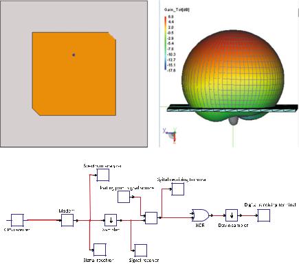
The antenna of the equipment 2 is modeled as shown in Fig. 6.8a, and the threedimensional far-field characteristics of antenna 2 are obtained by simulation as shown in Fig. 6.8b; the circuit of the equipment 2 is modeled as shown in Fig. 6.8c.

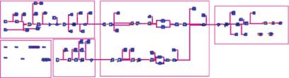
In the comprehensive simulation model in Fig. 6.9, the antenna simulation results, transmission channel model, and equipment behavioral circuit model of the two

(c)

Fig. 6.8 Equivalent model of equipment 2, a antenna model; b antenna pattern; c circuit model

equipment are comprehensively analyzed. Two aspects are required for the analysis, which are the “field” aspect and the “equivalent circuit” aspect. Using the “field” method, we can directly solve the system electromagnetic radiation problems according to Maxwell’s equations using the finite difference method, transmission line matrix method, moment method, and time-domain integral equation method. This kind of methods is theoretically strict; thus, the calculation results are accurate. However, the calculation time and memory requirements are relatively high in practical applications. The “equivalent circuit” method mainly refers to the circuit equivalent to the transmission model. With certain approximation, the mutual coupling relationship between equipment is simplified into an equivalent transmission module in circuit analysis by simplifying the coupling channel model and the radiation emission characteristics of the antenna. The transmission module is then converted into a circuit simulation module that can be imported into the circuit simulation to perform the complete analysis of the field of the system.

In the transmission module channel of Fig. 6.9, the isolation between equipment is calculated. It mainly includes two aspects: first, the calculation of the antenna gains

Transmitter 1

Receiver

Fig. 6.9 Field–circuit collaborative simulation model of equipment 1 and equipment 2

in the corresponding directions of the two antennas; and second, the calculation of the path attenuation. Then, the isolation can be expressed as Ltotal G1 − L + G2. The gain patterns simulated by the antenna 1 and the antenna 2 are, respectively, imported into the program, and according to the installed position (X1, Y1, Z1) of the antenna 1 and the installed position ( X, Y2, Z2) of the antenna 2, the antenna gain of the antenna 1 in the direction of the antenna 2 which is denoted as G1 and the gain of antenna 2 in the direction of antenna 1 which is denoted as G2 are calculated, respectively. Then, the spatial isolation between the antennas is calculated according to the type of the selected channel; thus, the isolation between the equipment is obtained. When the antenna needs local optimization, because the range for position adjustment is small, the change of the antenna gain pattern can be neglected. Therefore, the isolation between the two equipment after the position adjustment can be quickly obtained, and the scheme can be quickly adjusted accordingly. When the antenna needs to be adjusted in a large range of positions, it is necessary to reperform the field analysis, import the new gain pattern into the program, and then calculate the corresponding isolation.

The technology of directly incorporating the equivalent circuit model of the antenna into the system circuit model and participating in the system-level EMC simulation is still in research [16].

6.2.3 The Method of EMC Coordination Evaluation

After the interference prediction, if there is mutual interference between some RF equipment in the aircraft platform, the design scheme needs to be adjusted. In the adjustment, it is necessary to analyze the degree of mutual influence of these equipment, so as to identify equipment that requires more protection or suppression [67]. The DEMATEL method is a suitable system analysis method, which has been well applied in many fields; it is based on the matrix operation to obtain the mutual influence relationship, which matches the idea of interference correlation matrix in interference prediction. Thus, the DEMATEL method is used to analyze the influence degree and degree of being influenced by the equipment in the scheme. Through analysis, the main interference sources and susceptive equipment in the onboard RF

matrix. However, the operation of the DEMATEL method requires a square matrix, so the quantitative correlation matrix M needs to be expanded to the direct influence matrix D. The principle of expansion is as follows: The equipment set TR contains p transmitting equipment and q receiving equipment. The total number of equipment pieces in TR is n (equipment that is used both for transmitting and receiving is counted as 1 in TR). The matrix element of the existing equipment pair is the interference margin. When there is no equipment pair, the corresponding element is set to 0.

The direct influence matrix can be obtained by expansion as

Then, the comprehensive influence matrix T can be derived from the direct influence matrix D. The direct influence matrix D can be normalized to be

Then, the comprehensive influence matrix can be calculated as

T G(I − G)−1.

where I is the identity matrix.

(3)Tf is the vector describing the degree of influence the equipment has on others. Te is the vector describing the degree of influence the equipment gets. Tf and Te can be obtained from the comprehensive influence matrix T.

The influence degree of all equipment constitutes a vector Tf (Tf is the influence degree vector of the equipment, which represents the order of influence of the equipment on other equipment. It is used to determine the major interference source). Then, we can calculate the degree of influence the equipment Sj received using

vector Te (Te is a vector describing the degree of influence the equipment receives, which represents the order of the influence strength the equipment receives. It is used to determine the major susceptive equipment.).

4. Examples

There are 12 transmitting equipment and 17 receiving equipment in an aircraft. 11 of them are used both for transmitting and receiving and are denoted as {T R1 T R2 · · · T R11 }; there is one equipment that is only used for transmitting, which is denoted as {T1}; there are six equipment that are only used for receiving,

for the transmitting and receiving equipment, respectively. In the parameter list, the working frequency input is the central operating frequency of these equipment; the working bandwidth input is the maximum operating frequency range of the equipment; the transmitting power refers to the rated power, and the installed position refers to the location of the equipment on the same Cartesian coordinate system of the aircraft. The azimuth refers to the horizontal center direction of the main lobe of the antenna. The beam width of the azimuth refers to the lobe width of the antenna in the horizontal direction. The elevation angle refers to the vertical center direction of the main lobe of the antenna. The beam width of the elevation angle refers to the lobe width of the antenna in the vertical direction.

The transmitting equipment parameters and receiving equipment parameters in Tables 6.2 and 6.3 are imported into the software. Then, the interference residual is calculated for each equipment pair based on the hierarchical screening method, and the interference correlation matrix as shown in Table 6.4 is obtained.

In the interference correlation matrix, “Y” indicates no interference. There are three scenarios: (1) The equipment both transmits and receives, but does not interfere with itself; (2) there is not any possibility that the transmitting and receiving equipment overlap in spectrum based on the initial analysis of frequency, so they will not interfere with each other; (3) the two pieces of equipment do not overlap in the working time based on the working time analysis in the detailed screening, so the two pieces of equipment do not have the possibility of mutual interference.

The rest of the interference correlation matrix is the interference margin of the two pieces of equipment. The margin is calculated by amplitude filtering and corrected by frequency filtering. It can be seen from the interference correlation matrix that 204 pairs of transmitting and receiving equipment are formed by the RF equipment. Through calculation, we find that there are 24 equipment pairs that exhibited the possibility of interference, 3 pairs of equipment have critical interference, and 177 pairs do not interfere with each other. It can be seen that there is a lot of equipment with interference possibility, and the range of interference margin varied greatly. For this example, the results of the analysis are reasonable. It can be seen from the parameter list of the transmitting equipment and the receiving equipment that many pieces of equipment have a large working bandwidth, and the bandwidth here refers to in which the equipment can always work, rather than the bandwidth used for only one operation. For example, if the shortwave can work at 2–30 MHz, the working bandwidth in the list is 28 MHz, but the actual shortwave communication uses only a very narrow bandwidth. As a result, some pieces of equipment do not have fundamental interference in actual operation, but is determined to have fundamental interference as in the example. Therefore, the calculated interference margin is large, and there are many equipment pairs with possible interference. The interference margin for some equipment pairs is small because the interference level lower than the background noise has not been considered as the background noise level, but the theoretical value calculated from the model is used, which helps to determine the possibility of mutual interference of equipment.

Table 6.4 is the calculated interference correlation matrix C of the airborne RF equipment. Then, a numerical quantitative mapping is performed to obtain a quantitative correlation matrix M.

0 1 1 1 1 1 1 0 0 0 0 15 0 5 5 3 1 1 1 1 1 1 5

The size of the matrix M is 17 × 12, but the DEMATEL method is based on a square matrix, so the quantization correlation matrix M needs to be expanded to the direct influence matrix D. The principle of expansion is as follows: From the 12 pieces of transmitting equipment and 17 pieces of receiving equipment, the total equipment set TR is obtained. The total number of equipment pieces in TR is 18, which includes 11 transceivers, 1 transmitting only equipment, and 6 receiving only equipment. For the newly added transmitting–transmitting, receiving–receiving, and receiving–transmitting equipment pairs, we can get the direct influence matrix D by adding zeros, i.e.,

and the influence degree of all equipment constitutes the influence vector Tf . Then, we

and the degree of influence all equipment receives constitutes the influence vector Te. Then, there is

Te 0.36 1.33 0.98 0.88 1.47 1.00 0.85 0.70 0.64 0.68 0.68 0 0.04 0.64 1.00 1.25 0.64 1.44

From the equipment influence degree vector T f , it can be concluded that the equipment that has a serious influence on other equipment in the aircraft platform (i.e., the main equipment that causes the system to have EMC problems) are T R5, T R2, T R1, T1, T R3, T R4, and we need to take good control over their radiation. Similarly, it can be concluded from the influence degree vector Te that the equipment pieces that are more seriously affected by others (i.e., the equipment pieces that is more susceptive to the interference in the system) are T R5, R6, T R2, R4, which need to be in good protection.