


256 |
|
|
|
|
|
|
|
|
|
|
|
|
|
|
6 Application Cases of System-Level EMC Quantitative … |
|||||||||||||||||||||||||||||
|
|
|
|
|
|
|
|
|
|
|
|
|
|
|
|
|
|
|
|
|
|
|
|
|
|
|
|
|
|
|
|
|
|
|
|
|
|
|
|
|
|
|
|
|
|
|
|
|
|
|
|
|
|
|
|
|
|
|
|
|
|
|
|
|
|
|
|
|
|
|
|
|
|
|
|
|
|
|
|
|
|
|
|
|
|
|
|
|
|
|
|
|
|
|
|
|
|
|
|
|
|
|
|
|
|
|
|
|
|
|
|
|
|
|
|
|
|
|
|
|
|
|
|
|
|
|
|
|
|
|
|
|
|
|
|
|
|
|
|
|
|
|
|
|
|
|
|
|
|
|
|
|
|
|
|
|
|
|
|
|
|
|
|
|
|
|
|
|
|
|
|
|
|
|
|
|
|
|
|
|
|
|
|
|
|
|
|
|
|
|
|
|
|
|
|
|
|
|
|
|
|
|
|
|
|
|
|
|
|
|
|
|
|
|
|
|
|
|
|
|
|
|
|
|
|
|
|
|
|
|
|
|
|
|
|
|
|
|
|
|
|
|
|
|
|
|
|
|
|
|
|
|
|
|
|
|
|
|
|
|
|
|
|
|
|
|
|
|
|
|
|
|
|
|
|
|
|
|
|
|
|
|
|
|
|
|
|
|
|
|
|
|
|
|
|
|
|
|
|
|
|
|
|
|
|
|
|
|
|
|
|
|
|
|
|
|
|
|
|
|
|
|
|
|
|
|
|
|
|
|
|
|
|
|
|
|
|
|
|
|
|
|
|
|
|
|
|
|
|
|
|
|
|
|
|
|
|
|
|
|
|
|
|
|
|
|
|
|
|
|
|
|
|
|
|
|
|
|
|
|
|
|
|
|
|
|
|
|
|
|
|
|
|
|
|
|
|
|
|
|
|
|
|
|
|
|
|
|
|
|
|
|
|
|
|
|
|
|
|
|
|
|
|
|
|
|
|
|
|
|
|
|
|
|
|
|
|
|
|
|
|
|
|
|
|
|
|
|
|
|
|
|
|
|
|
|
|
|
|
|
|
|
|
|
|
|
|
|
|
|
|
|
|
|
|
|
|
|
|
|
|
|
|
|
|
|
|
|
|
|
|
|
|
|
|
|
|
|
|
|
|
|
|
|
|
|
|
|
|
|
|
|
|
|
|
|
|
|
|
|
|
|
|
|
|
|
|
|
|
|
|
|
|
|
|
|
|
|
|
|
|
|
|
|
|
|
|
|
|
|
|
|
|
|
|
|
|
|
|
|
|
|
|
|
|
|
|
|
|
|
|
|
|
|
|
|
|
|
|
|
|
|
|
|
|
|
|
|
|
|
|
|
|
|
|
|
|
|
|
|
|
|
|
|
|
|
|
|
|
|
|
|
|
|
|
|
|
|
|
|
|
|
|
|
|
|
|
|
|
|
|
|
|
|
|
|
|
|
|
|
|
|
|
|
|
|
|
|
|
|
|
|
|
|
|
|
|
|
|
|
|
|
|
|
|
|
|
|
|
|
|
|
|
|
|
|
|
|
|
|
|
|
|
|
|
|
|
|
|
|
|
|
|
|
|
|
|
|
|
|
|
|
|
|
|
|
|
|
|
|
|
|
|
|
|
|
|
|
|
|
|
|
|
|
|
|
|
|
|
|
|
|
|
|
|
|
|
|
|
|
|
|
|
|
|
|
|
|
|
|
|
|
|
|
|
|
|
|
|
|
|
|
|
|
|
|
|
|
|
|
|
|
|
|
|
|
|
|
|
|
|
|
|
|
|
|
|
|
|
|
|
|
|
|
|
|
|
|
|
|
|
|
|
|
|
|
|
|
|
|
|
|
|
|
|
|
|
|
|
|
|
|
|
|
|
|
|
|
|
|
|
|
|
|
|
|
|
|
|
|
|
|
|
|
|
|
|
|
|
|
|
|
|
|
|
|
|
|
|
|
|
|
|
|
|
|
|
|
|
|
|
|
|
|
|
|
|
|
|
|
|
|
|
|
|
|
|
|
|
|
|
|
|
|
|
|
|
|
|
|
|
|
|
|
|
|
|
|
|
|
|
|
|
|
|
|
|
|
|
|
|
|
|
|
|
|
|
|
|
|
|
|
|
|
|
|
|
|
|
|
|
|
|
|
|
|
|
|
|
|
|
|
|
|
|
|
|
|
|
|
|
|
|
|
|
|
|
|
|
|
|
|
|
|
|
|
|
|
|
|
|
|
|
|
|
|
|
|
|
|
|
|
|
|
|
|
|
|
|
|
|
|
|
|
|
|
|
|
|
|
|
|
|
|
|
|
|
|
|
|
|
|
|
|
|
|
|
|
|
|
|
|
|
|
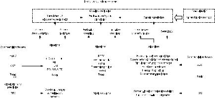
Fig. 6.1 Function framework of the system-level EMC quantitative design and evaluation software
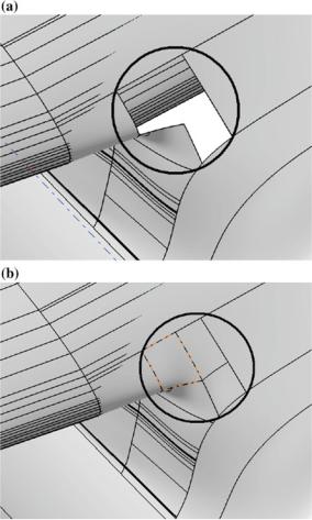
defect. If the precision defect is topological, then the model can be fixed by reintersection and topological reconstructing. If the precision defect is geometric, the surface must be fixed by modifying the mathematical definition of the geometric object, as shown in Fig. 6.2.
2.Structure Processing and Optimization of Electromagnetic Model used by Moment Method
The electromagnetic model for simulation analysis using moment method (MoM) can be obtained by building the electromagnetic model of the antenna, chamfering the geometric structure, and equivalenting typical radiation source and material. Then, structure processing and optimization can be performed toward the electromagnetic model.
When the MoM is used for simulation, structure processing and optimization of the electromagnetic model can be done as follows:
(1)Dipole and other linear antennas are all suitable to be equivalent to line model.
(2)Minimize geometry chamfering; if inevitable, simplify the chamfering properly during the electromagnetic modeling process.
(3)The triangulation patch model of the surface should follow the minimum criterion based on the square sum of the difference between any two sides as much as possible.
(4)When using the multi-level fast multi-pole algorithm (MLFMA), the iterative residuals of 0.01 is enough to meet the general engineering requirements.
(5)When choosing the integral equation, the combined field integral equation is preferred. If the target does not satisfy the closed condition, we should fill the target properly to make it applicable to the combined field integral equation. The combined factor could be other than 0.02.
6.1 EMC Geometric Modeling Method for Aircraft Platform |
257 |
Fig. 6.2 Model comparison before and after fixing,
a before fixing; b after fixing
(6)Typical antenna excitations, such as dipoles, can be simulated using discrete ports.
3.Structure Processing and Optimization Method of Electromagnetic Modeling for the Physical Optics Simulation
When building the electromagnetic model using high-frequency approximation method, if the electrical size of the local structure in the model does not conform to the precondition of the high-frequency approximation method, a large error would occur. Therefore, small structures in the model (such as small electronic equipment on the aircraft) can be simplified or ignored, because they do not satisfy the precondition of the high-frequency method and will bring in unnecessary densified grids for description in calculation.
258 6 Application Cases of System-Level EMC Quantitative …
When using the high-frequency method, small structures can be simplified or ignored based on the following assumption of physical optics: The curvature radius of the object on the surface is much larger than the incident wavelength.
When the wavelength of the electromagnetic wave is very short and the spatial variation of the mediums is slow enough, it can be assumed that the properties of the electromagnetic wave field in the local region are the same as those in the homogeneous medium. This way, the local wave surface of the electromagnetic wave is equivalent to the wave surface of a plane wave.
Specifically, the sphere can be used as a reference target for discrimination. For a sphere, its radius of curvature equals to its own radius. Therefore, the maximum size should satisfy D ≥ 10λ0. That is to say, when solving the scattering problem for electromagnetic wave of 10 GHz, small structures with a maximum size of 0.3 m could all be ignored from the target.
The structure processing and optimization method of electromagnetic modeling for simulation and analysis when using high-frequency approximation method (which is mainly physical optics method) could be summarized as follows: (1) Small structures could be simplified or ignored;
(2) The identification of small structure is based on the inference of the first basic hypothesis in physical optics √ρ >> √λ0 .
6.2Quantitative Evaluation Methods for System-Level EMC
6.2.1Interference Pair Determination and Interference Calculation
First, a coarse evaluation between antennas is carried out [57]. The purpose of the coarse evaluation is to eliminate the transceiver pairs that are clearly free of interference, thereby reducing the work required for the detailed evaluation in the next stage. The basic method is to perform simulation evaluation using a conservative simulation model and a loose electromagnetic emission limit.
Then, the method of screening by levels is adopted to predict EMC. It consists of two parts: (1) one-to-one transmission/receiving equipment pair prediction; that is, by calculating the interference margin between each transmitting and receiving pair, we can determine whether the interference margin meets the requirements and predict whether there is mutual interference between the two pieces of devices; (2) multi-to-one intermodulation interference prediction; that is, we analyze the working frequency bands of each piece of equipment in the platform, focusing on the interference of two signals and three signals intermodulation to decide whether the intermodulated signal will interfere with the receiver, as shown in Fig. 6.3.
6.2 Quantitative Evaluation Methods for System-Level EMC |
259 |
||||||||||||||||||||||
|
|
|
|
|
|
|
|
|
|
|
|
|
|
|
|
|
|
|
|
|
|
|
|
|
|
|
|
|
|
|
|
|
|
|
|
|
|
|
|
|
|
|
|
|
|
|
|
|
|
|
|
|
|
|
|
|
|
|
|
|
|
|
|
|
|
|
|
|
|
|
|
|
|
|
|
|
|
|
|
|
|
|
|
|
|
|
|
|
|
|
|
|
|
|
|
|
|
|
|
|
|
|
|
|
|
|
|
|
|
|
|
|
|
|
|
|
|
|
|
|
|
|
|
|
|
|
|
|
|
|
|
|
|
|
|
|
|
|
|
|
|
|
|
|
|
|
|
|
|
|
|
|
|
|
|
|
|
|
|
|
|
|
|
|
|
|
|
|
|
|
|
|
|
|
|
|
|
|
|
|
|
|
|
|
|
|
|
|
|
|
|
|
|
|
|
|
|
|
|
|
|
|
|
|
|
|
|
|
|
|
|
|
|
|
|
|
|
|
|
|
|
|
|
|
|
|
|
|
|
|
|
|
|
|
|
|
|
|
|
|
|
|
|
|
|
|
|
|
|
|
|
|
|
|
|
|
|
|
|
|
|
|
|
|
|
|
|
|
|
|
|
|
|
|
|
|
|
|
|
|
|
|
|
|
|
|
|
|
|
|
|
|
|
|
|
|
|
|
|
|
|
|
|
|
|
|
|
|
|
|
|
|
|
|
|
|
|
|
|
|
|
|
|
|
|
|
|
|
|
|
|
|
|
|
|
|
|
|
|
|
|
|
|
|
|
|
|
|
|
|
|
|
|
|
|
|
|
|
|
|
|
|
|
|
|
|
|
|
|
|
|
|
|
|
|
|
|
|
|
|
|
|
|
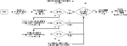
Fig. 6.3 Interference matrix generation process based on hierarchical screening prediction technology
1. Model and method of fast screening
The main purpose of the fast screening is to make a preliminary judgment from the frequency point of view, delete the transmitting/receiving pairs that do not interfere with each other, and predict the type of interference that may exist in the transmitting/receiving pairs, such that we can provide evidence for model selection for the interference margin calculation in the amplitude screening. According to our experience of EMC engineering design, when performing fast screening, the following frequency limit assumptions for transmitter and receiver are made:
(1)Assume the minimum spurious frequency of the transmitter is ( fT )min, and it can be denoted as 0.1 × fT .
(2)Assume the maximum spurious frequency of the transmitter is ( fT )max, and it can be denoted as 10 × fT .
(3)Assume the minimum spurious frequency of the receiver is ( fR )min, and it can be denoted as 0.1 × fR .
(4)Assume the maximum spurious frequency of the receiver is ( fR )max, and it can be denoted as 10 × fR .
Based on the above assumptions, the following judgments can be made:
(1)If | fT − fR | < 0.2 × fR , there is a fundamental interference margin;
(2)If 0.1 × fR < fT < 10 × fR , there is a transmitter interference margin;
(3)If 0.1 × fT < fT < 10 × fT , there is a receiver interference margin;
(4)If 0.1 × fT < 10 × fR or 0.1 × fR < 10 × fT , there is a clutter interference margin;
where fT is the transmitter center frequency and fR is the receiver center frequency.
2. Model and method of amplitude screening
The purpose of the amplitude screening is: Based on the amplitude of the interference signal, calculate and analyze the interference margin between the transmitting source and the susceptive device, remove as many obvious noninterference conditions as
260 |
6 Application Cases of System-Level EMC Quantitative … |
possible, perform frequency screening on equipment with large interference margins, and correct the interference margins. Interference margins appear in four forms: fundamental interference margin (FIM), transmitter interference margin (TIM), receiver interference margin (RIM), and spurious interference margin (SIM).
When it is determined that there is interference according to the fast screening, the corresponding interference margin calculation is performed according to the type of interference. The fundamental interference margin level is first calculated. If the interference margin is less than the screening level, there is no need to calculate the other three cases because their margin is even lower. Conversely, if the interference margin of the fundamental interference exceeds −6 dB, the TIM and RIM need to be calculated. If either of the interference margins generated by either of them exceeds −6 dB, the SIM needs to be calculated. When expressed in dB, the model for calculating the interference margin is
I M PT + GT − LT R + G R − PR + C F |
(6.1) |
where PT is the transmitting power of the transmitting equipment T m at the transmitting frequency fT , and this indicator needs to be confirmed according to the transmitter design indicator; GT is the gain of the transmitting antenna at fT ; LTR is the isolation between the transmitting antenna and the receiving antenna, which can be calculated using an electromagnetic field calculation software. It can also be simplified to free space attenuation and get solved using the geodesic method; PR is the susceptibility threshold level of the receiver Rn when the receiving frequency is fT ; C F is the correction coefficient for the interference margin, which is not considered in the amplitude analysis. C F is set to zero in the amplitude screening and will be calculated in the frequency screening.
In order to calculate the interference margin, it is necessary to guild a transmitter model, an antenna model, a transmission model, and a receiver model. The models are built based on the baseband characteristics such that we can obtain the amplitude–frequency characteristics including harmonics and out-band characteristics. Then, we can calculate the value of each item in formula (6.1), and substitute it into the calculation to get the interference margin.
The isolation LTR is calculated using the geodesic method based on the minimum angle.
3. Model and method of frequency screening
Correction factor C F is confirmed in the following two cases:
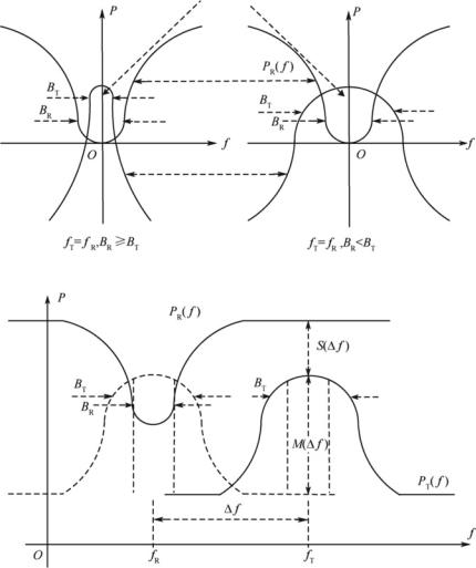
(1) Tuning. f ≤ (BT + BR )/2, where f | fe − fr |, BT is the 3 dB bandwidth of the transmitter, BR is the 3 dB bandwidth of the receiver. The tuning case is shown in Fig. 6.4a.
In this case, if the receiver bandwidth BR is greater than or equal to the transmitter bandwidth BT , then the correction factor C F is zero. If the receiver bandwidth BR is less than the transmitter bandwidth BT , then the calculation model for the correction factor C F is calculated using C F K log(BR /BT ) (dB), where K is the constant
6.2 Quantitative Evaluation Methods for System-Level EMC |
261 |
(a)
Receiving power
Receiver susceptibility threshold
Effective power
Receiving power = effective power |
Receiving power < effective power |
(b)
Receiver susceptibility threshold
Transmitting power
Fig. 6.4 Tuning and detuning, a tuning; b detuning
for a particular transmitting/receiving pair (when BR ≥ BT , or aligned with the same channel, K 0; when the noise-like signal of the RMS level is used, and BR < BT , there is K 10; when using the peak level of the pulse signal, and BR < BT , then K 20). (2) Detuning. When f > (BR + BT )/2, i.e., the transmitter and receiver center frequency deviates, the diagram of the detuning is shown in Fig. 6.4b.
In this situation, the transmitter power can enter the receiver in two ways. The transmitter transmits a modulation sideband into the receiver at the primary response frequency. The correction factor is C Ft K log(BR /BT ) + M( f ) (dB),
262 6 Application Cases of System-Level EMC Quantitative …
where M( f ) is the modulation sideband level (dB) above the transmitter power at the frequency interval f ; K is the same as the tuning case. The power of the transmitter’s main output frequency enters the receiver’s detuned response, and then C Fr ( f ) −S( f ) (dB), where S( f ) is higher than the receiver’s selectivity (dB) of the fundamental sensitivity when the frequency interval is f . The correction factor added to the interference margin model is C F max(C Ft , C Fr ).
4. Models and methods of detailed screening
The main purpose of the detailed analysis is to analyze the electromagnetic interference effects (such as intermodulation) of each piece of equipment and consider the corresponding receiver desensitization and other factors.
Intermodulation interference means that two or more signals are mixed at a nonlinear component to produce new signal frequency components that can be amplified and detected if they are close enough to the receiver’s tuning frequency. The mechanism is the same as functional signals and thus may cause performance degradation. They are equivalent to a linear combination of integer multiples of each signal frequency, and the interference frequency is predictable.
Desensitization means that when the receiver receives one or more strong nonfunctional signals in a channel adjacent to the tuning frequency of the receiver, the nonlinearity of the front end of the receiver causes the gain of the functional signal to decrease.
The signal-to-noise ratio without interference is
S/N PD − PR E F + (S/N )R E F (dB)
where PD is the function signal level (dBm); PREF is the reference signal level (dBm);
S N R E F is the signal-to-noise ratio of the reference signal level.
When the interfering signal power is greater than the saturation threshold of the receiver front end, the signal-to-noise ratio begins to decrease. The desensitization signal-to-noise ratio is
(S/N ) S/N − ( PA − PS AT )/ R(dB)
where S/N is the signal-to-noise ratio (dB) generated by the level of the functional signal without interference; PA is the power of the interference signal at the input of the receiver (dBm); PSAT is the saturation level of the receiver front end (dBm); R is the rate of desensitization.
The saturation level of the receiver front end is
PS AT PB + 10l g( f / fO R )
where PB is the saturation reference power (dBm) of the receiver; f / fO R is the interference transmission frequency interval relative to the receiver’s tuning frequency.
The amount of desensitization is
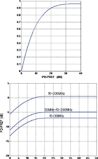
6.2 Quantitative Evaluation Methods for System-Level EMC |
263 |
(a)
Slope R
(b)
Saturated based power (dBm)
Fig. 6.5 Desensitization rate and saturation reference power curve, a desensitization rate; b saturation reference power curve