

48 3 Antenna Theory and Engineering
Therefore, the electromagnetic power carried by the main part of far-field region will be fully radiated. The amount of field in the far field that is inversely proportional to rS is called the radiation field
In the electromagnetic field, apart from the bounded field and the radiation field, there is another item proportional to 1 rS2, which is generally referred to as the inducted field.
3.2 Basic Antenna Concepts
This section introduces several basic concepts of the antenna [1], including directivity function, antenna pattern, radiation power, radiation resistance, main lobe, half-power beamwidth (HPBW), antenna side lobe, antenna gain, and antenna feed system.
3.2.1 Directivity Function and Pattern
In the radiation field of the alternating electric dipole, the electromagnetic field amplitude changes in accordance with sin θ . When θ 0 and θ π , the radiation field of alternating electric dipole is zero, and it is the strongest when θ π/2. It shows that the electromagnetic radiation generated by the alternating electric dipole is directional.
The directivity function is often used to indicate the directivity of the radiator. The directivity function F(θ , φ) is defined as
F(θ , φ) |E(θ , φ)| |Emax|
where |E(θ , φ)| is the amplitude of the radiation electric field in the direction (θ , φ), and |Emax| is the amplitude of the radiated electric field in the direction of the maximum radiation field.
The directivity function of the alternating electric dipole is F(θ , φ) |sin θ |. The representation of the directivity function in space is the antenna pattern. For
alternating electric dipoles, the curve of F(θ , φ) is quite like the number “8” on the plane where φ is constant. Since it only contains the electric power line of the radiation field on this plane, it is often called the E-plane. On the plane where F(θ , φ) is a circle, only the magnetic field lines of the radiation field are contained. Therefore, the plane is often called the H-plane.
3.2 Basic Antenna Concepts |
49 |
3.2.2 Radiation Power
The electromagnetic power radiated by the alternating electric dipole can be calculated from its field. With the alternating electric dipole as the center, using rS as a radius to make a closed sphere A, then the electromagnetic power through the surface A is
˙ |
A |
˜ |
· |
da |
P |
|
S |
|
˜
where S is the complex Poynting vector.
The radiated power of the alternating electric dipole can be calculated from the
far field |
|
|
|
|
|
|
|
|
|
|
|
|
|
|
P |
π η I 2dl2 |
|
|
|
|
|
|
|
|
|
||||
˙Σ |
|
|
|
(W) |
|
|
|
|
|
|||||
|
|
3λ2 |
|
|
|
|
|
|||||||
For alternating electric dipoles in |
|
free space, |
the wave |
impedance is η0 |
||||||||||
120π (Ω ). Therefore, the radiation power is |
|
|
|
|
|
|
|
|
|
|
||||
P |
2 |
I |
2 |
dl |
λ |
0 |
|
2 |
(W) |
|
|
|
|
|
˙Σ 40π |
|
|
|
|
|
|
|
|
2. dl |
|
||||
Obviously, the total radiation power is proportional to |
dl |
λ0 |
|
λ0 is often |
||||||||||
called the electrical size of an alternating electric |
dipole. For alternating electric |
|||||||||||||
|
|
|
|
|
||||||||||
dipoles, the electrical size is always small. Therefore, its radiation capacity is quite limited.
3.2.3 Radiation Resistance
Radiation resistance measures the radiation capacity of a radiator. Here, the term “resistance” in circuit theory is used to reflect the radiation of the radiator; that is, the power radiated by the radiator is equivalent to the power absorbed by a resistor, and this equivalent resistance value is defined as the radiation resistance of the radiator. Thus, when the current fed to the antenna by the transmitter is fixed, the bigger the radiation resistance of the antenna is, the stronger the radiation capability is. Referring to the form of the circuit formula, the radiation power PΣ is
PΣ I 2 RΣ 2(W)
The radiation resistance of the alternating electric dipole in free space is
RΣ 80π 2 dl λ0 2( )

50 |
3 Antenna Theory and Engineering |
Since the electrical size of the alternating electric dipole is small, its radiation resistance is quite small, which indicates that its radiation capability is not strong. For example, in free space, when dl λ0 0.1, it is already a very large electrical size for the alternating electric dipole, but the radiation resistance RΣ is only 7.89 .
3.2.4 Antenna Beamwidth and Gain
This section will introduce main lobe, half-power beamwidth (HPBW), side lobe, antenna gain, and so on closely related to EMC design. When analyzing the difference between the characteristics of the bare antenna and the characteristics of the installed antenna, we need to pay special attention to the large influence of the fuselage on the antenna pattern after the antenna is installed in the EMC calculation. Then, we can further explain the change of the antenna pattern caused by the fuselage and analyze the influence of the fuselage on the working distance of the installed antenna system.
1. Antenna pattern
The radiation of the transmitting antenna is not uniform in all directions of the space, and the energy received by the receiving antenna in all directions of the space is not uniform either. The direction selectivity of the antenna can be described by the antenna pattern [9].
The main lobe and its beamwidths, side lobes, and back lobes of the antenna can all be obtained from the antenna pattern.
(1)Main lobe is defined as the lobe with the highest radiation intensity in the pattern.
(2)The main lobe beamwidth is defined as the angular separation between the points at which the main lobe power drops to half the peak on the pattern, i.e., the angle between the 3 dB points.
(3)Side lobes are defined as other lobes than the main lobe.
(4)Back lobes are defined as lobes in the opposite direction of the main lobe.
2. Gain
The power gain is a variable describing the ability of the antenna to concentrate energy in a certain direction.
The power gain of an antenna is usually defined as the value of the gain at peak direction of the antenna’s main lobe. When the input power of antenna A is Pin (A), its main peak value is Pout (A). When using nondirectional reference antenna B with peaks Pout (B) Pout (A), the input power of B is Pin (B). Then, the power gain of antenna A is
D(θ , φ) |
Pin (B) |
(3.3) |
Pin (A) |
The bare antenna characteristics are defined as antenna characteristics before the antenna is installed (on another platform).
3.2 Basic Antenna Concepts |
51 |
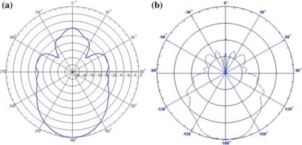
Fig. 3.1 Change of the antenna pattern before and after the installation of an antenna. a The antenna pattern before installation; b the antenna pattern after installation
The characteristics of the installed antenna are defined as the integrated antenna characteristics after the secondary radiation caused by the new electromagnetic boundary generated on the surface of the fuselage, after the bare antenna is installed.
Generally, the boundary of the fuselage makes the performance of the antenna characteristics of the bare antenna decrease. This drop is manifested in the radiation characteristics (directionality, gain, etc.) and impedance characteristics of the antenna. Figure 3.1 shows the change of the antenna pattern before and after the installation of an antenna.
The fuselage often makes the pattern of the airborne antenna become somehow “fat,” which means that the antenna’s working distance decreases, and the energy outside the main direction increases; as a result, the antenna isolation between the antenna and other antennas on the same aircraft decreases, and the mutual interference increases. Therefore, in the design and evaluation of EMC of the whole aircraft, it is necessary to consider the change of the antenna characteristics after the bare antenna is installed.
The following example illustrates the effect of the secondary radiation from the fuselage on the characteristics of the bare antenna [10].
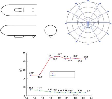
Figure 3.2 shows the effect of the gun bay of an aircraft on the radiation characteristics of the antenna. Since the fuselage and the gun bay are made of metal materials, the influence of the antenna toward the antenna pattern is relatively large. Figure 3.2b analyzes the influence of the distance between the antenna and the belly on the main lobe and the HPBW when the antenna is moved down in the vertical direction. Figure 3.2c analyzes the influence of the distance between the antenna and the gun bay on the main lobe and the HPBW when the antenna is moved in the backward direction. It can be seen that under certain conditions, the secondary radiation of the fuselage has a significant influence on the radiation characteristics of the airborne antenna.
52 |
|
3 Antenna Theory and Engineering |
(a) |
|
(b) |
Top view |
|
|
Aircraft body |
|
|
Gun bay |
Antenna |
Front view |
Side view |
|
|
(c)
Angle
Beamwidth -3dB position
Distance between antenna and gun bay / m
Fig. 3.2 Influence of a machine gun bay in the belly of an aircraft on the radiation characteristics of the antenna. a Aircraft fuselage; b the change of the antenna lobe in vertical direction; c the change of the antenna lobe in horizontal direction
3.2.5The Impact of Antenna Out-of-Band Characteristics Toward Aircraft EMC
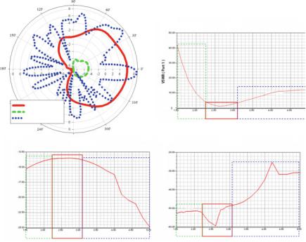
In the past, during the design of the airborne antenna and the analysis of the antenna layout of the whole aircraft, the influence of the out-of-band characteristics of the antenna has been rarely considered. However, with the increasing number of airborne antennas and the widening operation frequency band, the influence of the out-of- band characteristics of the airborne antenna (including the directional characteristics and the impedance characteristics) to the whole aircraft’s EMC cannot be ignored anymore. Figure 3.3a shows the pattern of an airborne antenna at the center operating frequency, at an out-of-band frequency point 1 lower than the center frequency, and at an out-of-band frequency point 2 higher than then center frequency. Figure 3.3b–d illustrates the change of the main lobe and side lobe of the airborne antenna at the
3.2 Basic Antenna Concepts |
53 |
(a)
(b)
Out-of-Band 1 |
Out-of-Band 2 |
|
In-Band |
In-Band |
|
|
|
Out-of-Band 1 |
|
|
Frequency |
Out-of-Band 2 |
|
|
|
|
|
|
|
(c) |
|
|
(d) |
dB (Total Gain) |
|
|
d B (Total Gain) |
Out-of-Band 1 |
In-Band |
Out-of-Band 2 |
Out-of-Band 1 |
|
|
||
|
|
|
Out-of-Band 2 |
|
|
|
In-Band |
|
|
Frequency |
|
|
|
|
Frequency |
Fig. 3.3 Airborne antenna characteristics with changes in frequency. a In-band and out-of-band pattern characteristics of an airborne antenna; b in-band and out-of-band SWR of an airborne antenna; c in-band and out-of-band main lobe characteristics of an airborne antenna; d in-band and out-of-band side lobe characteristics of an airborne antenna
center operating frequency, at an out-of-band frequency point 1 lower than the center frequency, and at an out-of-band frequency point 2 higher than then center frequency.
Figure 3.3a indicates that the change of pattern characteristics of the antenna inside and outside the operation band is very intense. Figure 3.3b–d shows that, if the out-of-band SWR does not increase rapidly (as Fig. 3.3b), the main lobe gain does not decrease rapidly (as Fig. 3.3c), and the side lobe gain increases rapidly (as Fig. 3.3d); thus, the effect of the out-of-band characteristics of the antenna on the whole antenna isolation cannot be ignored. Taking Fig. 3.3 for example, the ratio of the main and side lobes of the antenna within the operating band is about 25 dB. However, at the frequency point 2–3 times of the center frequency, the ratio of the main and side lobes has reduced to 2.5 dB and the SWR is 10. The antenna is therefore suffering from EMC problems.
A large number of practical problems have shown that when the EMC design accuracy requirements are high, the influence of the out-of-band characteristics of the antenna on EMC needs to be considered.