

26 |
2 Microwave Technology |
difficult to directly solve the electromagnetic field, the “microwave equivalent circuit theory,” using the thought called “changing field into circuit,” has gradually formed, with inspiration from the equivalent circuit method in the low-frequency circuit.
2.1 The Theory of Microwave Transmission Line
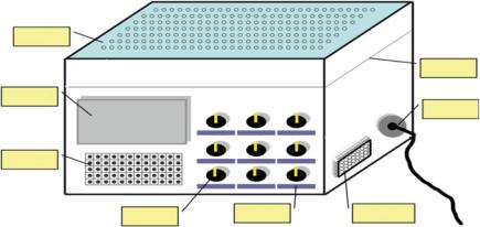
In EMC research, “case shielding” seems to be a perennial problem. The effective design of cases for the required shielding performance involves concepts of “singleconductor transmission line” and “double-conductor transmission line” in microwave technology.
In Fig. 2.1, the screen, vents, and slits have single-conductor effect, while the power lines, data lines, buttons, and switches have double-conductor effect.
2.1.1 Overview of Microwave Transmission Line
In the low-frequency case, it is sufficient to transfer energy from the power source to the load with two wires, and there are no special requirements for the form of the wires. However, when the wave frequency is very high, the distance between the two wires is comparable to the wavelength such that the energy is radiated into the space through the wire. In other words, the two wires act as antennas to a certain extent. To avoid the radiation loss, the transmission wires should be packed in a closed form like coaxial lines. As the frequency of the waves further increases, new problems arise: The optimal working state of a coaxial line is single-mode operation, and the outer diameter of the coaxial line is limited by the single-mode working condition
Vent hole
Slot
Screen
Power line
Keyboard
Switches |
Buttons |
Data line |
|
|
Fig. 2.1 Single-conductor and double-conductor effects in a typical case
2.1 The Theory of Microwave Transmission Line |
27 |
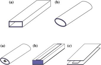
Fig. 2.2 Typical single-conductor transmission line. a Rectangle waveguide and b circular waveguide
Fig. 2.3 Typical double-/multi-conductor transmission lines. a Coaxial line; b microstrip line; and c stripline
(there is an optimal ratio between the inner and outer diameters of the coaxial line). When the frequency is high, the cross-sectional dimension of the coaxial line must be reduced. As a result, the field strength between the inner and the outer conductors increases under the same voltage and may easily cause breakdown, which limits the transmission power of the coaxial lines. Therefore, the operating frequency and transmission power of the coaxial line are quite limited.
Theoretical research shows that waveguides are characterized by low loss, large power capacity, and high operating frequency, but its working frequency band is much narrower than that of the coaxial lines.
The waveguide transmission line is constituted of a single conductor, so we call it as single-conductor transmission line. The coaxial line is composed of two conductors inside and outside, so it is called a double-conductor transmission line. The commonly used single-conductor microwave transmission line is rectangular waveguide and circular waveguide, as shown in Fig. 2.2. Double-conductor transmission lines include coaxial lines and microstrip lines, as shown in Fig. 2.3a, b. The stripline in Fig. 2.3c is a multi-conductor transmission line.
2.1.2Transmission State and Cutoff State in the Microwave Transmission Line
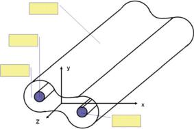
Figure 2.4 shows a columnar uniform transform system with a cross section of arbitrary shape. A uniform transmission line means that the cross section of the transmission line system is equal everywhere, and arbitrary shape means that the cross section can be in any shape. It can be seen from Fig. 2.4 that this case may be
28
Fig. 2.4 Columnar uniform transmission line system with arbitrary shape
2 Microwave Technology
Metal
Metal
Air
Metal
constituted by a plurality of transmission line conductors. For the sake of simplicity, it is assumed that metal under vacuum is an ideal conductor.
We will solve the electromagnetic wave existing in the transmission line system. The expression for the electromagnetic field of the cross section in the transmission
line system can be determined as
T2E(x, y) + kc2E(x, y) 0 |
|
T2H(x, y) + kc2H(x, y) 0 |
(2.1) |
where kc is the cutoff wave number, kc2 k2 + γ 2, k is the phase constant in free space, and γ is the propagation constant. The relationship between k, the wavelength λ, and the frequency f is:
k 2π λ 2π f c
kc is an important special parameter, and λc corresponding to kc is called the cutoff wavelength, λc 2π kc; the corresponding frequency is defined as cutoff frequency,
and fc c λc ckc |
2π. |
|
|
|
|
|
|
|
|
|
|
|
|
|
|
|
|
|
|
|
|
||
The propagation constant can be expressed as |
|
|
|
|
|
|
|
|
|
||||||||||||||
|
|
|
|
|
|
|
|
|
|
|
|
|
|
|
|
|
|
|
|
|
|
|
|
|
|
|
|
kc |
2 |
|
|
2π |
|
λ |
2 |
|
2π f |
|
fc |
|
2 |
|
|||||
γ α + jβ kc2 − k2 k |
|
− 1 |
|
− 1 |
|
− 1 (2.2) |
|||||||||||||||||
|
|
|
|
|
|
|
|
|
|
|
|
|
|
||||||||||
|
k |
|
|
λ |
|
λc |
c |
|
|
f |
|
||||||||||||
where α is the attenuation constant and β is the phase constant.
When kc is a positive real number, there are two distinct cases in the transmission line system shown in Fig. 2.4, namely the transmission state and the off state.
1. Transmission state
When λ < λc or f > fc, λ jβ is a pure imaginary number, and the solution of Maxwell’s equations in the transmission line system is
2.1 The Theory of Microwave Transmission Line |
29 |
||
E(x, y, z, t) |
|
E(x, y)e−j(ωt βz) |
(2.3) |
|
|
|
|
This solution indicates that there is a fluctuation process, and (ωt β z) indicates that there are electromagnetic waves transmitted in the +z- and -z-directions in the transmission line. The phase constant is
|
2π |
|
|
|
|
2 |
|
2π f |
|
|
|
|
2 |
|
|
β |
λ |
− 1 |
fc |
− 1 |
(2.4) |
||||||||||
|
|
|
|
|
|
|
|
|
|
||||||
λ |
|
λc |
c |
|
|
f |
|
||||||||
We usually take λ < λc or f > fc as the propagation conditions of the wave.
2. Cutoff state
When λ > λc or f < fc, λ α is a pure real number, and the solution of Maxwell’s equation in the transmission line system is
E(x, y, z, t) |
|
E(x, y)e αz e− jωt |
(2.5) |
|
|
|
It shows an in situ vibration process with only an axial attenuation field in the transmission line and no wave propagation. The attenuation constant is
|
2π |
|
λ |
2 |
|
2π f |
|
|
|
|
2 |
|
||
α |
|
− 1 |
fc |
− 1 |
(2.6) |
|||||||||
λ |
|
|
λc |
|
c |
|
|
f |
|
|||||
We usually take λ > λc or f < fc as the cutoff conditions of the wave, i.e., the cutoff wavelength and the cutoff frequency.
2.1.3The Concept of TEM Mode, TE Mode, and TM Mode in Microwave Transmission Line
In Fig. 2.4, z-direction is the longitudinal direction of the microwave transmission line system, i.e., the propagation direction of energy transmission line; x–y-direction is the transverse direction of the microwave transmission line, i.e., perpendicular to the direction of the energy transmission of the transmission line. Since the traveling wave in the microwave transmission line system satisfies Maxwell’s equation, in general, the lateral component and the longitudinal component of the distribution function in the transmission line are not independent of each other.
From the expression of the distribution function, the guided waves can generally be divided into the following three categories:
(1)Transverse electric wave (TE wave): The characteristic is that the longitudinal
component of the electric field is zero, and the longitudinal component of the magnetic field is not zero, i.e., Ez 0 and H z 0.
30 |
2 Microwave Technology |
(2)Transverse magnetic wave (TM wave): The characteristic is that the longitudinal
component of the electric field is not zero, and the longitudinal component of the magnetic field is zero, i.e., Ez 0 and H z 0.
(3)Transverse electromagnetic wave (TEM wave): It is characterized that the lon-
gitudinal component of the electric field and the longitudinal component of the magnetic field are both zero, i.e., Ez 0 and H z 0.
Characteristic difference of TEM wave from the TE wave and the TM wave: When the longitudinal components of the electric field and the magnetic field are both zero, in order to obtain a nonzero solution, there must be kc 0, which means fc 0. It shows that in the case of TEM waves, the cutoff frequency is zero, so the TEM electromagnetic waves of all frequencies are in a propagating state.
Since Ez 0 and H z 0, the distribution function becomes a two-dimensional vector of only x and y.
Note: TEM waves cannot be transmitted by any system. For example, in a hollow waveguide, since the TEM wave does not satisfy the Maxwell equation, there will not be any TEM wave in the hollow waveguide. However, in a double-conductor or multi-conductor transmission line system, TEM waves can exist.
In circuit theory, the ratio of voltage to current has an impedance dimension, which represents the transfer state of energy. In microwave technology, due to the distribution characteristics of the system, we use the ratio of electric field to magnetic field to describe the state of energy transfer, and the ratio also has an impedance dimension.
For TE waves, the wave impedance is
|
|
|
|
|
|
|
|
|
|
|
|
|
|
|
|
|
1 |
|
|
|
|
|
|
|
|
|
|
|
|
|
|
1 |
|
|
|
|
|
|
|
|
|
||||||||
|
|
ωμ0 |
|
|
|
μ0 |
|
|
|
|
|
|
|
|
|
|
|
|
|
|
|
|
|
|
|
|
|
|
|
|
|
|
|
|
|
|
|||||||||||||
η |
TE |
|
|
|
|
|
|
|
|
|
|
|
|
|
|
|
|
|
|
|
|
|
|
|
|
|
|
|
120 π |
|
|
|
|
|
|
|
|
|
( |
) |
(2.7) |
||||||||
|
|
|
|
|
|
|
|
|
|
|
|
|
|
|
|
|
|
|
|
|
|
|
|
|
|
|
|
|
|
|
|
|
|||||||||||||||||
|
|
β |
|
|
|
ε0 |
|
|
|
|
λ |
|
2 |
|
|
|
|
|
|
|
|
|
λ |
2 |
|
|
|
||||||||||||||||||||||
|
|
|
|
|
|
|
|
|
|
|
|
|
|
|
|
|
|
|
|
|
|
|
|
|
|
1 − |
|
|
|
|
|
||||||||||||||||||
|
|
|
|
|
|
|
|
|
|
|
|
|
|
|
|
|
|
|
|
|
1 − |
|
|
|
|
|
|
|
|
|
|
|
|
|
|
|
|
|
|
|
|
|
|
|
|
|
|||
|
|
|
|
|
|
|
|
|
|
|
|
|
|
|
|
|
|
|
|
|
λc |
|
|
|
|
|
|
|
|
|
|
|
|
|
λc |
|
|
|
|
|
|
||||||||
For TM waves, the wave impedance is |
|
|
|
|
|
|
|
|
|
|
|
|
|
|
|
|
|
|
|
|
|
|
|
|
|||||||||||||||||||||||||
|
|
|
|
|
|
|
|
|
|
|
|
|
|
|
|
|
|
|
|
|
|
|
|
|
|
|
|
|
|
|
|
|
|
|
|
|
|
|
|
|
|
|
|
|
|
|
|||
|
|
|
|
β |
|
|
|
|
|
|
|
|
|
|
|
|
|
λ |
|
2 |
|
|
|
|
|
|
|
λ |
2 |
|
|
|
|
|
|||||||||||||||
|
|
|
|
|
|
|
|
|
|
|
|
|
|
|
|
|
|
|
|
|
|
|
|
|
|||||||||||||||||||||||||
|
|
|
|
|
|
μ0 |
|
|
|
|
|
|
|
|
|
|
|
|
|
|
|
||||||||||||||||||||||||||||
|
ηTM |
|
|
|
|
|
|
|
|
|
|
|
|
|
1 − |
|
|
|
|
|
|
|
|
120π |
|
1 − |
|
|
|
|
|
|
( |
|
) |
(2.8) |
|||||||||||||
|
|
ωε0 |
|
|
|
|
ε0 |
|
|
|
λc |
|
|
|
|
|
|
λc |
|
|
|
|
|
|
|||||||||||||||||||||||||
For TEM waves, the wave impedance is |
|
|
|
|
|
|
|
|
|
|
|
|
|
|
|
|
|
|
|
|
|
|
|||||||||||||||||||||||||||
|
|
|
|
|
|
|
|
|
|
|
|
|
|
|
|
|
|
|
|
|
|
|
|
|
|
|
|
|
|
|
|
|
|
|
|
|
|
|
|
|
|
|
|
|
|
|
|
||
|
|
|
|
|
|
|
|
|
|
|
|
|
|
|
|
|
|
|
|
|
|
|
|
|
|
|
|
|
|
|
|
|
|
|
|
|
|
|
|
|
|
|
|
|
|
|
|||
|
|
|
|
|
|
|
|
|
|
|
|
|
|
|
|
|
|
|
β |
|
|
μ0 |
|
|
|
|
|
|
|
|
|
|
|
|
|
|
|
|
|||||||||||
|
|
|
|
|
|
|
|
ηTEM |
|
|
|
|
|
|
|
|
|
120 π ( ) |
|
|
|
|
|
|
|
|
|
(2.9) |
|||||||||||||||||||||
|
|
|
|
|
|
|
|
ωε0 |
|
|
|
|
ε0 |
|
|
|
|
|
|
|
|
|
|
||||||||||||||||||||||||||