

1.1 The Physical Meaning of Maxwell’s Equations |
7 |
enclosed by the curved surface. In other words, the charge is the source of the electric flux density vector.
4.Physical meaning of Gauss’s law for magnetism
In free space, the net magnetic flux that passes through any closed curved surface is zero; that is, there is no source magnetic charge of the magnetic flux density vector.
5.Physical meaning of the law of charge conservation
For a system of volume V and external surface S, the net charge in the system changes only when there is charge in or out. If the system has no charge exchange with the outside world, that is, the system is a charge-closed system, then the net charge within the system is constant. In other words, the charge can only be transferred in the form of current, but cannot be generated or disappeared by itself.
1.1.5 The Overall Physical Meaning of Maxwell’s Equations
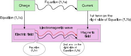
The significance of Maxwell’s equations in the electromagnetic field theory is the same as the significance of Newton’s laws of mechanics in theoretical mechanics. Any real electromagnetic field behavior obeys Maxwell’s equations. In the scope of nonrelativity, the behavior of electromagnetic fields must obey Maxwell’s equations in integral form. From the form of the equations, Maxwell’s equations describe the relationship between the electromagnetic field quantities E and H and their source quantities ρ, J, which is illustrated in Fig. 1.1, where the arrow “ →” indicates direct relationship, and “~~ → ” indicates a time-varying relationship.
Of all the relationships reflected in Maxwell’s equations, there are two situations that need further discussion.
Fig. 1.1 Overall physical meaning of the electromagnetic field law
8 |
|
|
|
|
|
1 Electromagnetic Field and Wave |
|
|
|
|
|
|
|
|
|
|
|
|
|
|
|
|
|
|
|
|
|
|
|
|
|
|
|
|
|
|
|
|
|
|
|
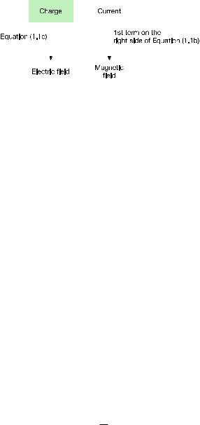
Fig. 1.2 Overall physical meaning of EMF laws when all physical variables are nontime varying
(1)All physical variables are time invariant. At this time, the relationship between the field quantities E and H and their source quantities ρ and J is shown as Fig. 1.2. The electromagnetic field law at this time is:
S E · d s 0 |
(1.2a) |
||
C H · d s |
S J · d a |
(1.2b) |
|
S ε0 E · d a |
V ρ d V |
(1.2c) |
|
S μ0 H · d a 0 |
(1.2d) |
||
S |
J · d a 0 |
(1.2e) |
|
…
In this case, there is no mutual coupling between E and H. Only two sides of “→” can be retained in Fig. 1.1. This situation is a static (or nontime-varying) electromagnetic field issue.
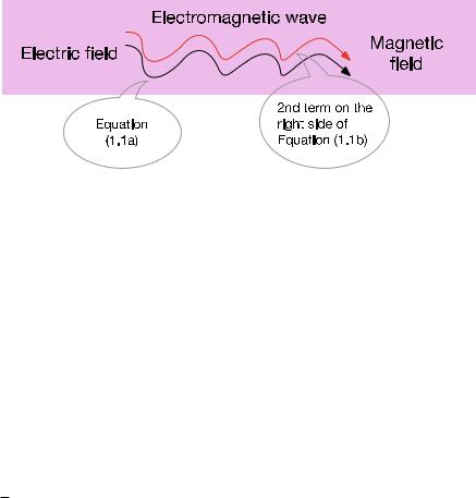
2.Source quantities are zero, i.e., ρ 0, J 0. In this situation, the expression of the relationship between the electromagnetic field quantities E and H and their source quantities ρ and J is shown in Fig. 1.3. The electromagnetic field law in this situation can be written as
d |
|
C E · d s − dt S μ0 H · d a |
(1.3a) |
1.1 The Physical Meaning of Maxwell’s Equations |
9 |
|||||
|
|
|
|
|
|
|
|
|
|
|
|
|
|
|
|
|
|
|
|
|
|
|
|
|
|
|
|
Fig. 1.3 Overall physical meaning of EMF law when the source quantities are zero
|
d |
|
|
C H · d s |
|
S ε0 E · d a |
(1.3b) |
dt |
|||
S ε0 E · d a 0 |
(1.3c) |
||
S μ0 H • d a 0 |
(1.3d) |
||
From Fig. 1.3, we see that in the region without charge and current, the timevarying electromagnetic field can still exist through mutual coupling, and this form of existence is called the electromagnetic wave. Free space is a typical medium for electromagnetic wave propagation.
Now, we further explain |
C H · d s |
|
d |
S ε0 E · d a. After transformation, the |
||||||
|
dt |
|||||||||
formula can be rewritten as |
C H · d s |
d |
S ε0 E · d a |
S |
∂ |
(ε0 E) · d a. |
∂ |
ε0 E |
||
dt |
|
∂ t |
∂ t |
|||||||
and the current J satisfies the same equation in generating magnetic field in form. ∂∂t (ε0 E) is added to electromagnetic field law by Maxwell for the mathematical integrity. This term is called the displacement current term. After adding this item to Ampere’s law and combined with Faraday’s law of electromagnetic induction, the existence of electromagnetic waves is theoretically proved. At first, people only thought that this was a mathematical treatment because there was no experimental evidence of the existence of electromagnetic waves. It was not until 1888, nine years after Maxwell’s death, that Hertz’s electromagnetic experiments proved the genius prophecy of Maxwell.
The purpose of revisiting the overall physical meaning of Maxwell’s equations is to provide our reader systematical explanation that the characteristics of the electronic circuits in DC (frequency 0 Hz) or low frequency (frequency < 100 kHz) and the characteristics of the electronic circuits in RF (frequency > 1 MHz) or microwave (frequency > 1 GHz) are essentially different.
Now, we explain the above with examples.