Fig. 4.14 Factors affecting the isolation between transmitter and receiver

profile reflects the product’s response to electromagnetic emission and describes the susceptibility of the susceptive object. The isolation is to ensure that the interference profile of the interference source does not intersect with the susceptibility profile of the susceptive object, and it has a certain segmentation degree of isolation required by the margin; the safety margin is to prevent the vulnerability of the product due to its susceptibility, and it sets safety margin requirement to the vulnerable points and its surroundings.

4.3.5 Equipment Isolation

Equipment isolation is proposed relative to antenna isolation. Antenna isolation calculation is one of the most important topics in the system-level EMC analysis and prediction. The antenna isolation requirement is directly related to the installation position of the airborne antenna and may even affect the geometric layout and performance design of the transceiver system.

In practical applications, however, it is not rare that airborne transceiver systems that have met the design requirements for antenna isolation still suffer from mutual interference problems. After long-term investigations, we found that one of the main reasons leading to this problem is that the antenna isolation only serves as an intermediate parameter in the EMC design of the transceiver system, and it does not fully reflect the EMC of the transmitter and receiver; i.e., the antenna isolation only isolates between transmitting antenna—spatial channels—and receiving antenna. However, the factors affecting the EMC between transmitter and receiver also include the receiver’s receiving characteristics, the transmitter’s transmission characteristics, and the connectors and cables connecting the receiver/transmitter to the receiving/transmitting antenna. Moreover, the nonlinearity of the RF front end, out-of-band characteristics, bonding characteristics of the cable and connector, and shielding characteristics all contribute to EMC issues between transmitter and receiver.

In order to describe the EMC of the transceiver system accurately and improve the effectiveness of the prediction and design, it is necessary to investigate the isolation of the equipment. The factors affecting the isolation between the transmitter and the receiver are shown in Fig. 4.14.

Spatial isolation between the transmitting and receiving antennas needs to be calculated first, no matter if we are solving antenna isolation or equipment isolation.

Spatial isolation, antenna isolation, and equipment isolation, and the relationship among the three are defined as follows.

(1)Spatial isolation: Assuming that both the receiving antenna and the transmitting antenna are omnidirectional point source antennas, the isolation between the two antennas is spatial isolation, which reflects the contribution of various boundary conditions of isolation points.

(2)Antenna isolation: Receiving gain of the receiving antenna and the transmitting gain of the transmitting antenna after installation are included on the basis of spatial isolation. The influence of the aircraft fuselage needs to be taken into consideration when we calculate the receiving gain of the receiving antenna after installation. Similarly, the transmitting gain of the transmitting antenna after installation is also affected by the aircraft fuselage. In the antenna isolation, the transmitting and receiving antennas are usually directional, and the directionality is affected by the aircraft fuselage where the antennas are installed.

(3)Equipment isolation: Based on the isolation of the antenna, the characteristics of the RF front end of the receiver, the characteristics of the connector and the connecting cable between the receiver and the receiving antenna, the characteristics of the transmitter RF front end, and the characteristics of the connector and connection cable between the transmitter and the transmitting antenna are taken into account.

4.3.6 Quantitative Allocation of Indicators

Quantitative allocation of indicators refers to the implementation of the overall technical requirements of the system into equipment/subsystems.

Quantitative allocation of indicators is usually based on the principle of the three aspects of EMC, namely electromagnetic emission, electromagnetic susceptibility, and isolation.

For instance, the equipment isolation between the transmitter and the receiver is 180 dB. After subtraction of the isolation between the transmitting antenna and the receiving antenna (the isolation caused by the pattern, polarization and antenna position of receiving antenna and the transmitting antenna), the isolation between the EMI source and the susceptive equipment should be no less than 110 dB (the isolation requirement on the left side of Fig. 4.15a). Based on the actual capabilities of EMI sources and susceptive equipment, the indicators can be allocated through the following five ways.

(1)The out-of-band emission attenuation of the interference shall not be less than 85 dB, and the suppression capability of susceptive equipment to the out-of- band emission of the interference source shall not be less than 25 dB, as shown in Fig. 4.15a.

(2)The out-of-band emission attenuation of the interference source should not be less than 85 dB, but the suppression of out-of-band emissions from the

(e)

Fig. 4.15 Quantitative allocation of system-level EMC indicators

susceptive equipment to the interference source can only reach 20 dB. Therefore, the relative layout of the interference source and susceptive equipment needs to be adjusted to provide an additional 5 dB of spatial isolation; i.e., the isolation requirement between the EMI source and the susceptive equipment needs to be modified to “no less than 105 dB,” as shown in Fig. 4.15b.

(3)The out-of-band emission attenuation of the interference source can reach 82 dB but cannot reach 85 dB. Meanwhile, the maximum suppression capability of susceptive equipment to the out-of-band emission of the interference source can only reach 25 dB. Then, the system needs to provide an extra 3 dB spatial isolation by adjusting the relative layout of interference source and susceptive

equipment; i.e., the isolation requirement between the EMI source and the susceptive equipment needs to be revised to “no less than 107 dB,” as shown in Fig. 4.15c.

(4)The suppression capability of the susceptive equipment to the out-of-band emission of interference sources can only reach 20 dB, but the out-of-band emission attenuation of the interference source has the potential to achieve 90 dB, which is equivalent to the transmission equipment sharing 5 dB indicator for susceptive equipment, as shown in Fig. 4.15d. Similarly, if the transmitting equipment has insufficient capacity but the susceptive equipment has potentials, the susceptive equipment should share the indicator for the transmitting equipment.

(5)The out-of-band emission attenuation of the emission source can reach 82 dB but cannot reach 85 dB; the suppression capability of susceptive equipment to the out-of-band emission of the interference source can reach 20 dB but cannot reach 25 dB. Under this condition, the solution is either to allocate the indicators that the transmitting equipment and susceptive equipment cannot achieve to the system or to reduce the isolation requirements. It is worth noticing that decreasing isolation requirements means reducing performance, as shown in Fig. 4.15e.

4.3.7 The Construction of EMC Behavioral Model

The EMC behavioral model is proposed by the EMC Research Team of Beihang University to solve the top-level quantification, demonstration, and design of the system.

Equipment parameters and circuit design layout are often required when using simulation analysis software to do performance simulation analysis of the system, equipment, circuits, etc. However, it often happens that when the system is demonstrated at the top level, the subsystems and equipment in the system only have major functional indicators, but does not come with detailed design scheme, component parameters, or circuit design layout.

Based on the analysis and research of various state-of-the-art simulation technologies, this book proposes the concepts of system-level behavioral simulation model, subsystem/equipment behavioral simulation model, etc. [12].

The behavioral modeling of EMC targets to model the external characteristics (behavior), rather than the physical or internal structure of the system. This method focuses on the behavioral trends of the system and establishes homomorphism model through induction method. In other words, the informal description method is used to determine the main observation variables of the system. The observed data is then processed through induction and informal description. New data is then generated through extrapolation. The model data is thereby generated, and the system behavioral model is established. This method is called behavioral modeling.

The definition of behavioral modeling can be summarized as: modeling based only on the electromagnetic emission to the outside and the susceptive response

Fig. 4.16 Hierarchy of electronic system simulation model

to the external electromagnetic signal. With this method, the circuits and equipment within system, subsystems, and equipment are considered as a black box and internal characteristics are unnecessary to be extracted.

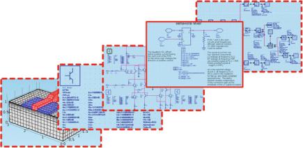
Figure 4.16 illustrates the electronic system simulation model hierarchy. The bottom layer is the physical model of the semiconductor structure. After the port parameters are extracted, device circuit models such as the transistor model are established, which are used to further build integrated circuit models such as amplifiers and mixers; the top layer is a complex system digital simulation model. The behavioral model is the bridge between the circuit model and the system simulation model. If the behavioral model is used to describe the subcircuit, the complexity of the system calculation problem caused by the existence of a large number of components can be avoided. This kind of behavior description will greatly improve the simulation speed and efficiency [16].

EMC behavioral simulation is the application of behavioral models to systemlevel EMC simulation. An electronic information system usually contains multiple subsystems and complex coupling relationships. By classifying and layering, the system can be divided into many subsystems with different functional characteristics, which are required for EMC analysis. Then, the behavioral model for the subsystems can be built one by one. The EMC behavioral modeling and simulation process are shown in Fig. 4.17. After the classification, the performance parameters of the subsystem are extracted, and a specific mathematical model is selected for description. During the modeling process, the model is continuously revised according to the performance verification, and the reliability of the model is thus improved. Finally, the model is used for system-level EMC simulation.

The EMC behavioral model has certain similarities with the behavioral model of analog electronic circuit devices, e.g., the large signal model and small signal model of semiconductor triodes. It is worth noticing that in the simulation of system EMC,