

5.3 EMC Modeling Methodology |
193 |
Fig. 5.59 Gray system behavioral model of the electronic system
Using the gray behavioral model, in the electronic system design stage, based on the precompliance test results, we can investigate the EMC problems existing in the equipment in a timely manner and formulate quantitative solutions, which effectively reduces the problem of excessive emission from the equipment in a later phase and reduces the interference between equipment. Thus, the product’s EMC quality can be improved.
5.4 EMC Simulation Method
The process of EMC simulation method is proposed as follows:
(1)EMC concept description based on equipment characteristics, which include:Sort the main radiation sources and susceptive equipment in the system, and mark the type of the equipment (transmitter, receiver, transceiver); sort the energy transmission relationships from the radiation source to the susceptive point through field, field–circuit, and circuit, and construct the system interference correlation relationship; list the factors affecting EMC in the interference correlation relationship; i.e., list the main EMC indicators for each equipment.
(2)Build the equipment’s EMC behavioral model. The modeling process mainly includes: using a formal modeling language and various modeling tools to quantify the conceptual model and establish an executable behavioral model covering the functions of the system. Two methods are used to create the behavioral model: (1) behavioral modeling based on equipment characteristics and
(2) behavioral modeling based on interference correlation matrix. The former adopts a graphical circuit language for simulation, and the latter uses an analytical mathematical expression for simulation.
194 |
5 Critical Techniques of Quantitative System-Level EMC Design |
|
Table 5.10 |
Antenna parameters |
|
|
|
|
Antenna mode |
Affiliated system and function |
|
|
|
|
Polarization mode |
Operation frequency and bandwidth |
|
|
|
|
Input impedance |
Standing wave ratio |
|
|
|
|
Installation position |
Having a radome or not |
|
|
|
|
Transmitting power |
Working principle |
|
|
|
|
Receiver sensitivity |
Dynamic range of receiver |
|
|
|
|
Feed mode |
|
Feed loss |
|
|
|
Antenna efficiency |
Equivalent aperture or height |
|
|
|
|
Phase center |
|
|
|
|
|
Structure size and characteristic parameters |
|
|
|
|
|
Out-of-band characteristics of antenna |
|
|
|
|
|
Beam characteristics of the E surface |
Beam characteristics of the H surface |
|
|
|
|
Half power beam width |
Half power beam width |
|
|
|
|
Main lobe gain |
Main lobe gain |
|
|
|
|
Side lobe gain |
Side lobe gain |
|
|
|
|
Depth at zero point |
Depth at zero point |
|
|
|
|
Beam width of the first zero point |
Beam width of the first zero point |
|
|
|
|
(3)Conduct EMC evaluation and performance optimization so that the system meets the EMC requirements.
We illustrate the EMC simulation process in detail using several cases.
5.4.1System-Level EMC Simulation Method for an Aircraft (Case 1)
When performing system-level EMC simulation, we often face problems of incomplete system/subsystem parameters or unknown operation mechanisms. Therefore, we need to collect equipment parameters, build basic models, and perform precompliance testing of design phase simultaneously.
1. Basic information collection
(1)Sort the system working principle and cross-linking relationship. Understand the use of the equipment, working principle, installation location, and input and output interfaces with other systems.
(2)Sort the cross-linked signal characteristics. Understand the input and output signal characteristics of the equipment and other systems, including: type, voltage, frequency, filtering mode of the power supply; operating mode, rotational speed of the motor; frequency, whether there is frequency division or frequency
5.4 EMC Simulation Method |
195 |
Table 5.11 Receiver parameters |
|
|
|
Communication equipment name |
Communication equipment code |
|
|
First LO frequency |
First LO bandwidth |
|
|
Second LO frequency |
Second LO bandwidth |
|
|
First IF frequency |
First IF bandwidth |
|
|
Second IF frequency |
Second IF bandwidth |
|
|
Working mode |
|
|
|
Selectivity (type, parameters specification, passband, and |
|
stopband of the filter) |
|
|
|
Gain and noise figure of the system amplifier |
|
|
|
Gain and noise figure of the system mixer |
|
|
|
Local oscillator crystal frequency |
|
|
|
Receiver sensitivity |
|
|
|
Demodulation method |
|
|
|
Isolation, out-of-band rejection, spurious, harmonics, etc. |
|
|
|
multiplication, frequency stabilization mode, out-of-band rejection, spurious, attenuation of each harmonic, etc., of the crystal oscillator; type, amplitude, waveform, bandwidth, modulation included or not, modulation characteristics, conduction mode, harmonic characteristics of the analog signal; waveform, amplitude, pulse width, frequency, bandwidth, duty cycle, repetition frequency of the digital signal; type, model, impedance, and other performance parameters of the transmission cable; type, location, and performance parameters of connectors.
(3)Analyze EMI threats. Understand the EMI threats of the equipment, its past and potential failures, and test items that are difficult to pass.
(4)Sort the conventional EMI prevention measures. Understand the EMC design measures taken and their effects, including: cable layout; layout of PCB board and board devices, circuits, routing; grounding and grounding resistance (grounding position and mode of the analog ground, digital ground, power ground, shielding ground, safety ground, etc.); filtering (including threats, filtering measures, expected results, and test results); shielding (including threats, shielding measures taken, expected results, and test results); lap joints (including lap handling and lap joint resistance); antenna parameter table (Table 5.10), receiver parameter table (Table 5.11), and transmitter parameter table (Table 5.12).
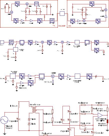
2. Basic model library
Establishing a behavioral simulation model library of commonly used airborne equipment is very useful for EMC simulation. The EMC models of common airborne equipment are shown in Fig. 5.60.
196 |
5 |
Critical Techniques of Quantitative System-Level EMC Design |
|
Table 5.12 |
Transmitter parameters |
||
|
|
|
|
Communication equipment name |
|
Communication equipment code |
|
|
|
|
|
First LO frequency |
|
First LO bandwidth |
|
|
|
|
|
Second LO frequency |
|
Second LO bandwidth |
|
|
|
|
|
First IF frequency |
|
First IF bandwidth |
|
|
|
|
|
Second IF frequency |
|
Second IF bandwidth |
|
|
|
||
Working mode, transmitting power, dynamic gain |
|
||
|
|
|
|
Modulation method |
|
|
|
|
|
||
Frequency points and the suppression of harmonics |
|
||
|
|
||
Filter (types, parameters, passband, and stopband) |
|
||
|
|
||
Gain and noise figure of the system amplifier |
|
||
|
|
||
Gain and noise figure of the system mixer |
|
||
|
|
||
The suppression of out-of-band, spurious, harmonics, etc. |
|
||
|
|
|
|
The equipment model library is mainly based on the design principle diagrams, working principle diagrams, and EMC test data of the subsystems and equipment. The equipment model is a functional description of the object. The model library parameter values can be filled and modified according to the test results of a different equipment. In order to ensure the accuracy and validity of the model, and to ensure that the model effectively includes all of the EMC failure factors, it is necessary to verify the model iteratively based on the test data.
3. Design precompliance test
In order to determine the EMC requirements and provide basis for EMC design, an overall design EMC test is required, including: analysis and test of electromagnetic environment, simulation test of equipment, subsystem and antenna optimal layout, and test for overall interference control.
(a)Shortwave radio;
(b)Microwave landing system;
(c)Ultrashort wave radio;
(d)Fuel gauge;
(e)TACAN;
(f)Airborne velocity radar;
(g)Airborne audio communication system;
(h)DSSS–QPSK communication system;
(i)Airborne GSM mobile communication system.
4.Conceptual description of EMC based on equipment characteristics
5.4 EMC Simulation Method |
197 |
By establishing a digital aircraft model, it is possible to analyze the interference relationships among the subsystems at the whole aircraft level, including the circuit–cir- cuit, circuit–field, and field-level interference/susceptive interference relationships of the interference/susceptive equipment. Then, we can build analysis model for subsystems, create the design signal flow and the interference signal flow, and predict
(a) |
(b) |
(c)
(d)
Fig. 5.60 EMC radiation quantification model for commonly used airborne equipment
198 |
5 Critical Techniques of Quantitative System-Level EMC Design |
(e)
(f)
(g)
Fig. 5.60 (continued)
5.4 EMC Simulation Method |
199 |
(h) |
(i) |
Fig. 5.60 (continued)
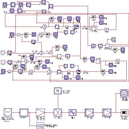
the radiation emission quantitatively to determine the interference the equipment suffers from by using the time-domain, frequency-domain, hybrid field, and field— circuit coupling coordination methods. Next, we can build a behavioral simulation model to analyze the factors affecting the EMC design and decompose the EMC indicators, such as shielding performance of transmitters and susceptive equipment, cable layout, distribution of electromagnetic environment, resonance characteristics of the cabin, equipment layout, tolerable degradation, equipment safety priorities, and safety margins of susceptive equipment. This way, we can complete the quantitative collaborative EMC design for the aircraft. Figure 5.61 shows the interference relationship of the electronic equipment of an aircraft, including over ten airborne equipment including shortwave radios, ultrashort wave radios, servo systems, fire control systems, integrated navigation, fuel gauges, and radio compasses.
200 |
|
|
|
|
|
|
|
|
5 Critical Techniques of Quantitative System-Level EMC Design |
||||||||||||||||||
|
|
|
|
|
|
|
|
|
|
|
|
|
|
|
|
|
|
|
|
|
|
|
|
|
|
|
|
|
|
|
|
|
|
|
|
|
|
|
|
|
|
|
|
|
|
|
|
|
|
|
|
|
|
|
|
|
|
|
|
|
|
|
|
|
|
|
|
|
|
|
|
|
|
|
|
|
|
|
|
|
|
|
|
|
|
|
|
|
|
|
|
|
|
|
|
|
|
|
|
|
|
|
|
|
|
|
|
|
|
|
|
|
|
|
|
|
|
|
|
|
|
|
|
|
|
|
|
|
|
|
|
|
|
|
|
|
|
|
|
|
|
|
|
|
|
|
|
|
|
|
|
|
|
|
|
|
|
|
|
|
|
|
|
|
|
|
|
|
|
|
|
|
|
|
|
|
|
|
|
|
|
|
|
|
|
|
|
|
|
|
|
|
|
|
|
|
|
|
|
|
|
|
|
|
|
|
|
|
|
|
|
|
|
|
|
|
|
|
|
|
|
|
|
|
|
|
|
|
|
|
|
|
|
|
|
|
|
|
|
|
|
|
|
|
|
|
|
|
|
|
|
|
|
|
|
|
|
|
|
|
|
|
|
|
|
|
|
|
|
|
|
|
|
|
|
|
|
|
|
|
|
|
|
|
|
|
|
|
|
|
|
|
|
|
|
|
|
|
|
|
|
|
|
|
|
|
|
|
|
|
|
|
|
|
|
|
|
|
|
|
|
|
|
|
|
|
|
|
|
|
|
|
|
|
|
Fig. 5.61 Interference relationship of electronic equipment of an aircraft
Fig. 5.62 EMC digital model of an aircraft
Figure 5.62 shows the EMC digital model of an aircraft.
5. EMC simulation analysis of equipment
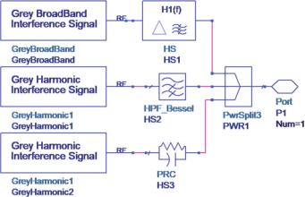
The equipment model can be modified, and the equipment’s EMC can be simulated according to the basic model and characteristics of the equipment. For example, the harmonics and broadband noise generated by the fundamental frequency of a shortwave radio can interfere with the highly sensitive receiving equipment (such as ultrashort wave radios) on board. For any frequency in the broadband, the final-stage transistor load of the shortwave radio power amplifier may not be in the best matching state and may work in the saturation region or the cutoff region, thereby causing a large nonlinear distortion and resulting in a series of harmonics and broadband noise. In order to formulate radio design requirement that meets the requirement of CE106, behavioral simulation methods are used to analyze equipment performance and reduce the harmonic rejection ratios. This way, the design requirements can be proposed.
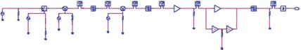
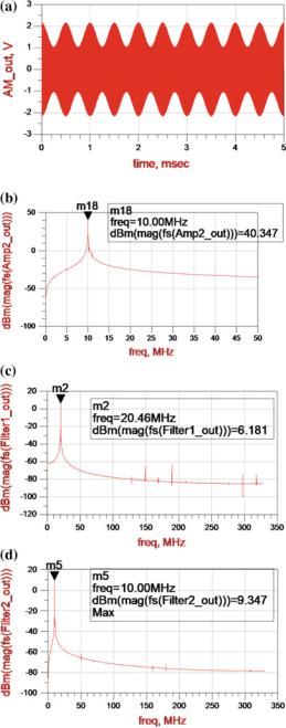
The behavioral model of shortwave radio emission is shown in Fig. 5.63. The characteristics of the output spectrum of the shortwave radio in the modeling and simulation are shown in Fig. 5.64.
5.4 EMC Simulation Method |
201 |
Probe
|
|
|
Modem |
|
Mixer |
Source |
Resistance |
Source |
Resistance |
Source |
Resistance |
Filter
Probe |
Probe |
Probe |
|
Mixer |
|
Source |
Filter |
Amplifier |
Resistance |
|
Probe
Resistance
Amplifier
Amplifier Amplifier
Filter
Resistance
Probe
Output
Attenuator
Fig. 5.63 Shortwave radio behavioral emission model
6. EMI simulation analysis between subsystems
Shortwave radios and ultrashort wave radios use adjacent frequencies, and out-of- band harmonics and broadband spurious interferences generated by shortwave radios may cause interference to ultrashort wave radios. The following section analyzes the interference of shortwave radios to ultrashort wave radios.
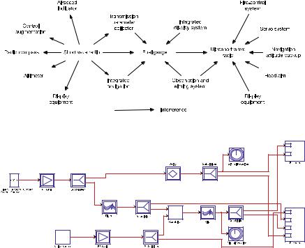
Based on the behavioral models of shortwave radios and ultrashort wave radios, a detailed model is established for single-frequency noise interference and broadband noise interference, and the interference characteristics of the two radios under various modes are analyzed. Ultrashort wave radio in the system uses two antennas and has two operating modes, AM and FM as shown in Fig. 5.65.
According to the above analysis, the network models that need to be established in the simulation analysis include shortwave models (including nonlinear power amplifier modules), ultrashort wave radio susceptibility models (AM and FM thresholds), and two antenna coupling modules. The specific simulation analysis content is shown in Table 5.13.
Table 5.14 provides the results of “interference on the ultrashort wave FM receiving system from the harmonic emission of the shortwave radio through ultrashort wave antenna 1” to determine if the design requirements are met based on whether the susceptibility threshold is exceeded.
5.4.2Out-of-Band Nonlinear Interference
Simulation Method for Transmitting and Receiving Systems (Case 2)
The traditional development of transmitting and receiving systems only takes into account the in-band parameters such as power gain, pattern, impedance, and radiation efficiency. Each piece of equipment is provided by a different vendor and has its own design specifications. It is rare if there is any systematic analysis on the influence other than the functional specifications, such as the out-of-band spurious and out-of- band susceptibility. Many problems have been found in the implementation of EMC engineering in recent years, and engineers have tried to systematically study the out-of-band characteristics of the equipment. Generally, multiple transmitters and receivers are distributed on the same platform. Although each transmitter or receiver
202 |
5 Critical Techniques of Quantitative System-Level EMC Design |
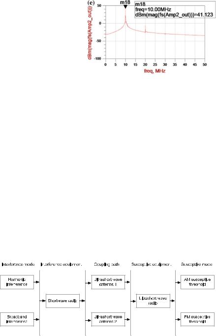
Fig. 5.64 Analysis of output spectrum characteristics of shortwave radio behavioral modeling and simulation,
a time domain output of the ideal model; b frequency domain output of the ideal model; c the first IF output; d the second IF output; and e nonlinear output through the nonlinear amplifier
Table 5.13 List of interference simulation decomposition between subsystems
Interference |
Interfering |
Coupling |
Susceptive |
Susceptive |
Content for simulation analysis |
equipment |
mode |
path |
equipment |
mode |
|
|
|
|
|
|
|
Shortwave |
Harmonic |
Ultrashort |
Ultrashort wave |
AM |
Interference on the ultrashort wave AM receiving system from the |
radio |
transmis- |
wave |
radio |
susceptive |
harmonic emission of the shortwave radio through the ultrashort wave |
|
sion |
antenna 1 |
|
threshold |
antenna 1 |
|
|
|
|
|
|
|
|
|
|
FM |
Interference on the ultrashort wave FM receiving system from the harmonic |
|
|
|
|
susceptive |
emission of the shortwave radio through the ultrashort wave antenna 1 |
|
|
|
|
threshold |
|
|
|
|
|
|
|
|
|
Ultrashort |
|
AM |
Interference on the ultrashort wave AM receiving system from the |
|
|
wave |
|
susceptive |
harmonic emission of the shortwave radio through the ultrashort wave |
|
|
antenna 2 |
|
threshold |
antenna 2 |
|
|
|
|
|
|
|
|
|
|
FM |
Interference on the ultrashort wave FM receiving system from the harmonic |
|
|
|
|
susceptive |
emission of the shortwave radio through the ultrashort wave antenna 2 |
|
|
|
|
threshold |
|
|
|
|
|
|
|
|
Broadband |
Ultrashort |
|
AM |
Interference on the ultrashort wave AM receiving system from the |
|
spurious |
wave |
|
susceptive |
broadband spurious emission of the shortwave radio through the ultrashort |
|
emission |
antenna 1 |
|
threshold |
wave antenna 1 |
|
|
|
|
|
|
|
|
|
|
FM |
Interference on the ultrashort wave FM receiving system from the |
|
|
|
|
susceptive |
broadband spurious emission of the shortwave radio through the ultrashort |
|
|
|
|
threshold |
wave antenna 1 |
|
|
|
|
|
|
|
|
Ultrashort |
|
AM |
Interference on the ultrashort wave AM receiving system from the |
|
|
wave |
|
susceptive |
broadband spurious emission of the shortwave radio through the ultrashort |
|
|
antenna 2 |
|
threshold |
wave antenna 2 |
|
|
|
|
|
|
|
|
|
|
FM |
Interference on the ultrashort wave FM receiving system from the |
|
|
|
|
susceptive |
broadband spurious emission of the shortwave radio through ultrashort |
|
|
|
|
threshold |
wave antenna 2 |
|
|
|
|
|
|
Method Simulation EMC 4.5
203

204
Table 5.14 Harmonic interference to ultrashort wave radio (125 MHz) from shortwave radio (25 MHz) |
|
|
|
5 |
|||||
Shortwave |
Harmonics |
Cable loss |
Isolation (dB) |
Noise of the |
Receiving |
Interference |
Exceeding the |
Interference |
Critical |
emission |
(dBm) |
(dB) |
|
the ultrashort |
suppression |
(dBm) |
threshold (dB) |
or not |
|
harmonic |
strength |
|
input end of |
out-of-band |
threshold |
|
|||
frequency |
|
|
|
wave (dBm) |
(dB) |
|
|
|
Techniques |
(MHz) |
|
|
−58.6 |
−10.7 |
|
−113 |
|
|
|
|
|
|
|
|
|
||||
f 0 |
50.9 |
3 |
80 |
23.3 |
Yes |
|
|||
2f 0 |
−11.2 |
3 |
−35.7 |
−49.9 |
80 |
−113 |
−16.9 |
No |
of |
3f 0 |
−14.5 |
3 |
−46.8 |
−64.6 |
80 |
−113 |
−31.6 |
No |
DesignEMCLevel-SystemQuantitative |
|
|||||||||
4f 0 |
−20.6 |
3 |
−48.7 |
−72.3 |
80 |
−113 |
−38.3 |
No |
|
5f 0 |
−21.5 |
3 |
−50.3 |
−74.8 |
0 |
−113 |
38.2 |
Yes |
|
5.4 EMC Simulation Method |
205 |
Fig. 5.64 (continued)
can meet the requirements of the EMC specification, the strong out-of-band signals of some devices in a limited space may still fall within the band of other devices. The out- of-band radiation characteristics may cause mutual interference between transmitters and receivers. In particular, some transmitters have large transmitting power and weak antenna directivity, and the omnidirectional power is easily received by other receivers on the same platform. Therefore, the out-of-band nonlinear interference characteristics have an important influence on the EMC of the entire platform.
In the simulation and analysis model of system-level EMC, in addition to the analysis of the functional signals, other signals with potential interference also need to be analyzed using the behavioral simulation methods. Therefore, it is necessary to establish a behavioral simulation model of the transmitter and the receiver, and fully consider the out-of-band performance of the system. Additionally, we need to focus on the sub-circuit modules with large influence, such as amplifiers and mixers, because they work in the nonlinear regions and their spurious products are likely to cause serious interference.
According to the active nonlinear out-of-band interference characteristics of the transmitters and receivers, the behavioral simulation method is used to establish the behavioral model of the transmitting and the receiving equipment. The spectral distribution of the transmitting equipment and the frequency response characteristics of the receiving equipment are analyzed to investigate the effects of nonlinear inter-
Fig. 5.65 Behavioral modeling, simulation, and analysis of interference between subsystems
206 |
5 Critical Techniques of Quantitative System-Level EMC Design |
ference signals from the transmitting system on other receiving equipment on the same platform. At the same time, we propose a method for the allocation of the third-order intermodulation distortion parameters with a large influence on system modeling and provide a modified cascaded model of the third-order intermodulation distortion parameters. Finally, we discuss a practical analog predistortion circuit that suppresses the third-order intermodulation distortion.
1. Out-of-band nonlinear interference of transmitters and receivers
An actual RF system needs nonlinear and active components including crystal diodes and bipolar transistors. It can be used for signal detection, mixing, amplification, frequency multiplication, switching, and so on. Nonlinear interference signals are also the result of signal modulation of amplifiers or mixers in nonlinear regions. It is a system-level interference phenomenon which usually occurs when the signal groups are large and the signals are easily coupled. In the process of EMC analysis, it is often found that each device in the system satisfies its own requirements, but problems still occur when integrated into the platform. Under certain circumstances, the radiation intensity of the transmitting equipment is still relatively strong and the energy of out-of-band radiation is likely to cause interference to susceptive equipment within a short distance. Additionally, the susceptive equipment itself may also cause unnecessary response due to the nonlinear characteristics.
(1) EMC interference prediction principle
The occurrence of any EMI follows the three aspects of EMI, and the interference prediction problem can be described by a general mathematical model. The interference model can be used to describe any interfering equipment with radiation emission characteristics in the system. Assuming the interference power output by the interference source is PT (t, f ), the influence of the propagation path on the interference signal is represented by the transfer function by T (t, f, r, θ ) (where t is time, f is frequency, r is distance, and θ is the propagation direction). Then, the effective power of the interference generated by the interference source at the susceptive equipment is PI (t, f, r, θ ), which can be expressed in decibels as [57]
PI (t, f, r, θ ) PT (t, f ) − T (t, f, r, θ ) |
(5.172) |
The susceptive model can be represented as any equipment with radiation susceptibility in the system. PS (t, f ) describes the radiation susceptive characteristics of the equipment coupled with external interference. In order to quantitatively express the degree of compatibility and incompatibility, the interference margin is defined as
M(t, f ) PI (t, f, r, θ ) − PS (t, f ) |
(5.173) |
The performance of susceptive equipment can be evaluated by M(t, |
f ): |
(1)If M(t, f ) > 0, the susceptive equipment will be interfered. The value of M(t, f ) indicates the intensity of the interference.
5.4 EMC Simulation Method |
207 |
(2)If M(t, f ) 0, the susceptive equipment is in a critical state of interference; that is, the equipment may be subject to interference, and the safety margin is zero.
(3)If −6 < M(t, f ) < 0, the susceptive equipment will not be interfered, but it is likely to be interfered.
(4)If M(t, f ) < −6, the susceptive equipment will not be interfered and can work safely and stably.
In practical applications, when the susceptive equipment is affected by n interference sources, (5.173) can be generalized to
|
n |
|
M(t, f ) |
PIi (t, f, r, θ ) − PS (t, f ) |
(5.174) |
|
i 1 |
|
Equation (5.174) is usually called the interference prediction equation, which is universal.
(2) Model of radiation characteristics of the transmitting equipment
In EMC analysis and design, besides the spectrum power distribution within the band of the transmitting equipment, we also need to understand the spectral power distribution of the out-of-band spurious and harmonics. Since the output powers of a different transmitting equipment are different, circuits with the same function in different devices will also be different. In this case, the spectrum allocation rule is generally described by a statistical method. Ideally, the spectral power distribution of the transmitting equipment can be expressed as [58]
Pt ( f ) |
|
P |
+ aδ |
|
, f |
L ≤ |
f |
≤ |
f |
|
(5.175) |
|
¯B |
, |
B |
f |
|
|
H |
||||
|
P |
|
< f |
L |
, f |
> f |
H |
||||
|
|
¯N |
|
|
|
|
|
|
|
||
where the parameters have the same explanation as in Eq. (5.71).
The expressions of the statistical mean of the fundamental radiation power and the standard deviation are
|
|
|
|
|
|
1 |
m |
|
|
|
|
|
P |
|
Pi |
|
|
(5.176) |
|||
|
|
|
|
|
|
|||||
|
|
|
¯B |
|
|
|
|
|||
|
|
|
|
|
m i 1 |
|
|
|
||
|
|
|
|
|
1 |
|
m |
|
|
|
|
|
|
|
|
|
|
− |
P )2 |
(5.177) |
|
|
|
|
m − 1 i 1 |
|||||||
δB |
|
|
|
|
|
|
P |
|
||
|
|
|
|
|
|
( ¯B |
|
i |
|
|
where Pi is the measured value of a single transmitter’s output power of the fundamental wave; m is the sampling number of the transmitter.
However, in engineering practice, due to the nonlinear effects of signal sources, power amplifiers, filters, and other electronic components in the transmitting equipment, the output power of the transmitting equipment is not completely limited to a
208 |
5 Critical Techniques of Quantitative System-Level EMC Design |
certain frequency or within a narrow band. Harmonic and parasitic radiation components also exist. The general mathematical expression of the harmonic radiation of the transmitting equipment is
P |
+ A lg N |
h |
+ B |
(5.178) |
Ph (Nh f0) ¯B |
|
|
|
where fB is the fundamental frequency; Nh is the number of harmonics; A and B are the harmonic suppression constant of the transmitting equipment.
Similarly, the average power of parasitic radiation is
p |
|
|
¯B |
|
|
B |
|
|
|
P |
( f ) |
|
P + A lg |
f |
f |
|
+ B |
|
(5.179) |
The radiation signal of a common transmission equipment is a signal modulated by different types, and the energy is mainly distributed in a frequency band near the fundamental wave. Therefore, the transmission power model is
P |
+ W ( f ) |
(5.180) |
P( f ) ¯max |
|
|
¯
where Pmax is the statistical mean of the maximum radiation power of the transmitting equipment, W ( f ) represents the relative value (dBc) of a certain spectrum component and the maximum transmitting power of the fundamental wave, and its expression is
W ( f ) |
|
W |
+ N |
lg( |
| f − fB | |
), ( f |
|
f |
i−1 |
, f |
|
; i |
|
[1, n]) (5.181) |
|
|
|||||||||||||
|
i |
i |
|
fi |
|
|
i |
|
|
|||||
where the parameters have the same explanation as in Eq. (5.74).
Similarly, for the harmonics and spurious components of other carrier frequencies, the modulation envelope can be taken into account in a similar manner of Eq. (5.181).
The model built based on priori data is generally more universal, but in the actual analysis process, due to the lack of data, it is not easy to derive an accurate radiation characteristics model for the emission equipment. Therefore, we need to use the behavioral simulation method of the circuit to build a behavioral simulation model of the transmitting equipment. For developed equipment, we can also obtain accurate radiation characteristics through testing.
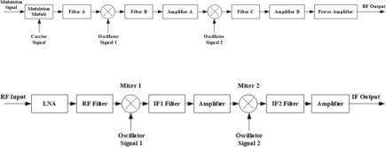
Figure 5.66 is a principle diagram of the RF end of a typical second-order superheterodyne transmitter. After the modulation signal and the carrier signal enter the modulation module, they go through the first-stage filtering and then enter the first mixer for mixing. After filtering and amplification, the modulation signal with higher frequency is obtained. Then, the signal enters the second mixer for frequency conversion. Next, the signal is filtered and amplified again. Finally, the signal is amplified by the power amplifier to obtain the radio frequency (RF) signal output.
The power of each frequency point calculated by the model can be expressed by the following expression (in decibels):
5.4 EMC Simulation Method |
209 |
Fig. 5.66 Principle diagram of the RF end of a typical second-order superheterodyne transmitter
Fig. 5.67 Principle diagram of the RF side of a typical second-order superheterodyne receiving equipment
Pt ( f ) Pin_sig ( f ) + Gt ( f ) + Lt ( f ) |
(5.182) |
where Pin_sig ( f ) is the spectral power distribution of the input signal for the transmitting equipment; Gt ( f ) is the total power gain of the amplifier and the mixer, which takes into account the nonlinear factor; Lt ( f ) is the total attenuation of the transmission power of the filter.
(3) Mode of receiving equipment response
At present, the sensitivity of the receiving equipment is getting higher, and the requirement of anti-interference ability of the external electromagnetic energy is becoming higher. When performing system EMC analysis and design, we need to focus on the frequency selection characteristics of the receiving equipment and the prediction of potential out-of-band signal. A block diagram of the RF end of a typical second-order superheterodyne receiver is shown in Fig. 5.67. Radio frequency (RF) signal enters the low-noise amplifier (LNA), passes the first-stage filtering, then enters the first mixer to be filtered and amplified, and then enters the second mixer for filtering and amplification, and finally the IF signal output is obtained.
Similarly, a generic model has also been formed for the receiving equipment based on a large amount of a priori data. The frequency selectivity of the receiving equipment near the operation bandwidth or in the main receiving channel can also be represented by a piecewise straight-line approximation [58].
S( f ) S( fi ) + Si lg( f / fi ) |
(5.183) |
where the parameters have the same explanation as in Eq. (5.78).
Signals located within the frequency points and frequency range outside the main receiving channel can also enter the receiver due to the system’s nonlinear characteristics, affecting the in-band of the receiving system. These frequencies or frequency bands are called additional receiving channels, which mainly include IF receiving
210 |
5 Critical Techniques of Quantitative System-Level EMC Design |
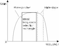
Fig. 5.68 Frequency selectivity of the superheterodyne receiving system
channel, image receiving channel, and harmonic receiving channel. The selective model of the receiving equipment in the main additional receiving channel is
S( fa ) I lg( fa fcen ) + J |
(5.184) |
where the parameters have the same explanation as in Eq. (5.79).
For an ideal receiver, the frequency selectivity should exhibit a rectangular characteristic. In reality, however, the selectivity of the receiving equipment is very different from the rectangular characteristics. In addition, due to the lack of sample data, it is difficult to use (5.184) to create an accurate frequency selective model of the receiving equipment. The full-band response characteristics of the receiving equipment can be analyzed using the behavioral simulation method of the circuit. For existing equipment, we can obtain more accurate response characteristics based on testing. The gain of the input RF signal after the entire RF system is
Gr ( f ) L f 1( f ) + L f 2( f ) + L f 3( f ) + · · · + L f n ( f ) + Gramp ( f )(dB) (5.185)
where Gr ( f ) is the gain of the entire system; L f n (n 1, 2, · · ·) is the attenuation value of the filter at all levels (negative in decibels); Gramp is the total gain of other modules such as the amplifiers and the mixers.
When the attenuation of L f n ( f ) is small in some frequency bands, Gr ( f ) will increase accordingly, and the fluctuant “wave packets” or the declining gradients in certain frequency bands are slower, as shown in Fig. 5.68. This phenomenon is particularly prominent in broadband receivers, because the interference signals of relevant frequencies are more likely to access receiving systems in complex electromagnetic environments.
Then, we set up a behavioral simulation model of the receiving equipment. The
calculated power at each frequency point can be expressed as |
|
Pr ( f ) PR F ( f ) + Gr ( f ) + Lr ( f ) |
(5.186) |
5.4 EMC Simulation Method |
211 |
where PR F ( f ) is the spectral power distribution of the weak signal received by the receiving equipment; Gr ( f ) is the total power gain of the amplifier and the mixer of the receiving equipment, of which the nonlinear factors need to be considered; Lr ( f ) is the total attenuation of the transmission power of the filter.
(4) Calculation of out-of-band nonlinear interference between equipment
For transmitting and receiving equipment, the product development regulations have corresponding requirements for their out-of-band characteristics. For example, CS103 specifies the requirements for intermodulation-conducted susceptibility of the antenna terminals, and the equipment cannot have intermodulation products that exceed the tolerance. CE106 specifies that the antenna terminal-conducted emission should not exceed the following values: All harmonic emissions and spurious emissions except the second and third harmonics of the transmitter (transmission state) should be at least 80 dB lower than the fundamental level; the second and third harmonics should be suppressed 50 + 10lgP (where P is the fundamental peak output power (W)) or 80 dB, whichever is less.
As long as the electronic equipment satisfies the national EMC regulations, it can be regarded as qualified. However, the method of tailoring national regulations is not necessarily effective, because when multiple pieces of electronic equipment are integrated into cascade, EMC problem will also appear. Even if the equipment satisfies the emission requirements, when it is positioned on the platform of a complex multi-set communication system, EMC problems may still occur. It is also easy to overlook the radiation interference caused by the nonlinearity outside the communication frequency band of the transmitting equipment. In general, only after the signal interference phenomenon outside the communication band of the transmitting equipment happened, will the engineers start to position the interference source through testing. This approach not only consumes a lot of human and material resources, but may also shorten the life of the equipment due to the large number of tests.
The power of the transmitting equipment is very large. Considering the power consumption, in order to ensure the efficiency of the transmitter output power, the power amplifier in the transmitting equipment is likely to work in the nonlinear area or even the saturation area, which will bring unnecessary harmonics and intermodulation products. Transmitting equipment and receiving equipment usually adopt the superheterodyne-type structure, the shortcoming of which is the production of the unnecessary spurious response during mixing. Therefore, the radiation interference outside the communication band caused by the nonlinearity cannot be ignored. The high-order harmonics and intermodulation products generated by the transmitting equipment are easily received by other highly susceptive receivers, affecting the normal reception of functional signals. The nonlinearity of the amplifier is usually described by gain compression and intermodulation distortion. The nonlinearity of the mixer is described by frequency conversion compression and intermodulation distortion. The nonlinear characteristic parameters have been discussed previously, including the output power P1dB of the 1 dB gain compression point, the input power PI I P3, and the output power PO I P3 of the TOI point.
212 |
5 Critical Techniques of Quantitative System-Level EMC Design |
||||
|
|
|
|
|
|
|
|
|
|
|
|
|
|
|
|
|
|
|
|
|
|
|
|
|
|
|
|
|
|
|
|
|
|
|
|
|
|
|
|
|
|
|
|
|
|
|
|
|
|
|
|
|
|
|
|
|
|
|
|
|
|
|
|
|
|
|
|
|
|
|
|
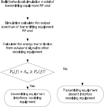
Fig. 5.69 Flowchart of out-of-band nonlinear interference prediction between communication systems
Out-of-band communication signals are the combination of several frequencies in a nonlinear circuit. The combined frequency can be expressed as m f1 + n f2 +l f3 + · · ·, where m, n, l, … are coefficients, and their values are 0,1,2,…. When m +n +l +· · · N , the N-th order signal is obtained. When there is only a single m or n equal to 2, 3, or larger value, the obtained signal will be second, third, or higher harmonics. After the signal passes through the mixer and amplifier, many harmonic signals and intermodulation signals appear. Especially in the mixing process, the power of the local oscillator required for the operation of the mixer is usually at least 10 dB greater than the power of the signal being processed; as a result, the local oscillator signal may have an energy re-injection effect on the generated out-of-band interference signal.
Large-scale electronic information platforms generally contain multiple sets of communication systems. High-power transmitters and high-sensitivity receivers are installed in a limited space which results in dense electromagnetic signals. For the communication systems on the same platform, EMI problems are easy to expose due to the close placement of the systems. System simulation can be used for prediction analysis from the interference transmitting system to coupled path and then to susceptive system, as shown in Fig. 5.69.
5.4 EMC Simulation Method |
|
213 |
Transmitting |
Receiving |
|
antenna gain |
antenna gain |
|
Transmission |
Tranceiving |
Receiving |
line loss |
antenna |
line loss |
|
spacial attenuation |
|
Output spectrum |
Receiving |
|
of transmitting equipment RF end |
equipment input |
|
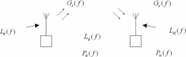
Fig. 5.70 Diagram of the energy transmission between transmitting and receiving equipment
First, we can build the behavioral model of the radio frequency of the transmitting system using circuit behavioral simulation. Considering the nonlinear characteristics of the amplifier and mixer module, we then calculate the out-of-band output spectrum of the transmitting system. The output spectrum includes various spurious components such as harmonics, intermodulation, and frequency conversion, some of which may fall within the communication band of other receiving systems. Then, we can filter out the interference frequency points that may fall into the communication band of other receiving systems and perform energy transmission calculation.
As shown in Fig. 5.70, the energy transmission relationship between the transmitting system and the susceptive system is
Pri ( fin ) Pti ( fin )Ltl ( fin )Gt ( fin )La ( fin )Gr ( fin )Lrl ( fin ) |
(5.187) |
Equation (5.187) can be written in the form of dB as |
|
Pri ( fin ) Pti ( fin ) + Ltl ( fin ) + Gt ( fin ) + La ( fin ) + Gr ( fin ) + Lrl ( fin ) |
(5.188) |
where fin is the operating frequency that can fall within the passband of the receiving system; Pri ( fin ) is the power coupled from the transmitting system to the susceptive system at a certain frequency in the receiving band; Pti ( fin ) is the out-of-band output signal power at the RF end of the transmitting system; Gt ( fin ) is the antenna power gain; La ( fin ) is the spatial attenuation; Gr ( fin ) is the receiver antenna power gain; Ltl ( fin ) is the transmitting line loss; Lrl ( fin ) is the receiving line loss;
In general, transmitting line loss Ltl ( fin ) and receiving line loss Lrl ( fin ) can be obtained by referring to the cable’s technical manual or through testing. The transmitting antenna power gain Gt ( fin ) and receiving antenna power gain Gr ( fin ) can be obtained through simulation software analysis or through testing. The spatial attenuation La ( fin ) can be calculated in the following two approaches:
(1)When the receiving antenna is located in the far-field area of the transmitting antenna

214 |
5 Critical Techniques of Quantitative System-Level EMC Design |
||
|
|
2D2 |
|
|
r > |
|
(5.189) |
|
|
||
λ
where D is the maximum size of the transmitting antenna, r is the distance between the transmitting antenna and the receiving antenna, and λ is the operating wavelength of the transmitted signal.
The spatial attenuation La ( fin ) (dB) of the transmitted signal between transmitting equipment and receiving equipment can be calculated by the following formula:
La 10 lg |
λ2 |
10 lg |
c2 |
(5.190) |
(4π )2r2 |
(4π )2r2 f 2 |
where f is the operating frequency (MHz) and c is the transmission speed of the transmitted signal (3 × 10⁸m/s).
Substituting π and c in (5.190), we get
La −27.56 + 20 lg f + 20 lg r |
(5.191) |
(2)When the distance r between the receiving antenna and the transmitting antenna satisfies
r ≤ |
2D2 |
(5.192) |
λ |
The spatial attenuation between the antennas can be obtained by testing or using existing calculation software. Generally, according to the actual antenna position, we can build the simulation model of the transmitting and the receiving antennas using electromagnetic field simulation software. Based on the model, we can calculate the spatial attenuation of the transmitted signal when it arrives at the susceptive equipment.
In different communication platforms, the diffraction attenuation, coupling shielding, and polarization mismatch between the transmitting and the receiving antennas vary greatly. Neglecting the above factors, we can calculate the radiation interference signal of the transmitting equipment falling into the passband of the receiving equipment of another communication system without considering the suppression of the received signal by the receiving equipment. Thus, the attenuation of the interference signal will not be affected by the above factors and reaches minimal; then, we can analyze the worst-case interference and predict more potential interfering frequencies. In general, the distance between the transmitting and the receiving antennas is short on the same platform, and the receiving antenna is usually located in the nearfield area of the transmitting antenna. The spatial attenuation La ( f ) of the signal between the transmitting equipment and the receiving equipment is calculated using field simulation software. In certain cases, La ( f ) can also be obtained by testing at the same time.
The determinant condition of the transmitting system interfering the receiving system is
5.4 |
EMC Simulation Method |
|
|
|
|
|
215 |
|||
Network Simulation and Analysis |
|
Interference Model of Short Wave Radio |
|
|||||||
|
|
|
|
|
|
|||||
|
|
Modem |
Mixer |
Filter |
Mixer |
Filter Amplifier |
Filter Amplifier |
Filter Amplifier |
||
Source |
Resistance |
Source Resistance |
Source |
Resistance |
|
Source |
Resistance |
|
|
Resistance |
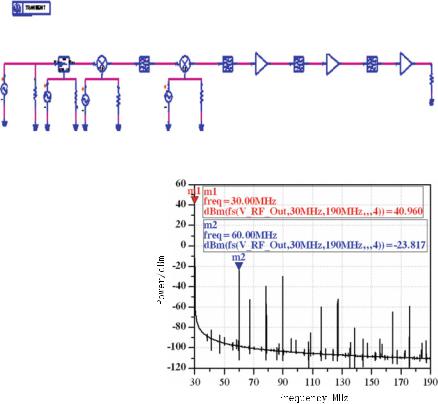
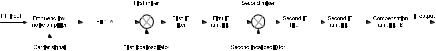
Fig. 5.71 RF end behavioral simulation model for the shortwave radio transmitting system
Fig. 5.72 Out-of-band output spectrum of the RF end of the transmitting system
Pri ( f ) + Sm ≥ Ps ( f ) |
(5.193) |
where Ps ( f ) is the sensitivity of the receiving system; Sm is the safety margin of the receiver (Sm is 6 dB in national regulation).
Now, we will analyze the interference of one shortwave radio (as a receiving system) from another ultrashort wave radio (as a transmitting system) in a real platform. The shortwave radio is a second-order superheterodyne structure as shown in Fig. 5.66. The modulated frequency is 512 kHz, the first local oscillator signal frequency is 12.466 MHz, and the second local oscillator signal frequency is 42.978 MHz. Thus, the output frequency is 30 MHz and the transmitting power is 12.5 W (40.96 dBm). Considering the nonlinear parameters of each module in the system, the simulation model of the RF end of the transmitting system is shown in Fig. 5.71.
The calculated spectrum range of the output is 30–190 MHz. Figure 5.72 shows the out-of-band output spectrum of the shortwave radio transmitter. The intensity of the signal at f 60 MHz is −23.817 dBm.
216 |
5 Critical Techniques of Quantitative System-Level EMC Design |
The operating frequency band of another ultrashort wave radio is 30–88 MHz, and the voice receiving sensitivity is not higher than 1.5 μV in the AM mode and 0.5 μV in the FM mode. We can use the signal source to simulate the voice signal, and transmit the FM signal to the RF end of the receiving system. Then, it can be found that when there is apparent whistle sound in the ultrashort wave radio headphone, the susceptibility at 60 MHz is −85 dBm.
The out-of-band radiation at 60 MHz for the shortwave emission system is selected from Fig. 5.72. In a communication platform in a limited space, the receiving antenna is usually located in the near-field area of the transmitting antenna. La ( f ) is provided by testing, and the value is 65.4 dB. In addition, through the technical manual, we get that Lti ( f ) equals 3 dB, Lri ( f ) equals 3 dB, Gt ( f ) equals 4 dB, and Gr ( f ) equals 3 dB.
It can be seen from Eq. (5.186) that Pri −88.217 dBm. According to (5.193), Pri ( f )+Sm −82.217 dBm (more than Ps −85 dBm). Therefore, we can conclude that on multiple communication platforms in a narrow space, ultrashort wave radios are also subject to radiation interference caused by the nonlinearity of the shortwave radio’s communication frequency band.
2. Research on intermodulation interference of transmitting and receiving systems
Among the many intermodulation parasitic products generated due to nonlinearity, the most typical and influential one is the third-order intermodulation (IM3) interference signal. The third-order intermodulation distortion signal is a powerful and difficult-to-filter-out parasitic product. When the receiver’s input signal contains two closely spaced frequencies ω1 and ω2, its third-order intermodulation distortion signal frequency ω ( ω 2ω1 − ω2) will fall into the receiving passband. Sinceω is very close to ω1 and ω2, the receiving of the desired signal will be interfered. This section analyzes the third-order intermodulation distortion parameters of each module in the receiving system EMC modeling and derives the method to calculate the amplitude of the third-order intermodulation output signal at all levels based on the distortion signal voltage in the worst case of the cascade circuit. Then, we also propose an allocation method of third-order intermodulation distortion parameters for each module of the receiving equipment using the constrained relationship of third-order intermodulation signal strength. Finally, we discuss an analog predistortion circuit suppressing the third-order intermodulation signal for later improvement of the product.
(1)The TOI point cascade equation in the model of the transmitting and receiving system
Transmitters and receivers generally consist of antennas, RF systems, and modulation or demodulation systems. The most popular superheterodyne RF systems include sub-circuits with nonlinear characteristics including amplifiers and mixers. Section 5.4.2 has discussed the characteristics of the amplifiers and the mixers operating in the nonlinear region and the parameters that describe the nonlinear character-
5.4 EMC Simulation Method |
217 |
Fig. 5.73 Spectrum component after a dual-tone signal enters the nonlinear equipment
istics. The following discussion focuses on the third-order intermodulation distortion parameters (TOI point). The TOI point fully describes the third-order intermodulation distortion degree of the nonlinear amplifier and the mixer.
Taking two continuous wave signals as input, the frequency of the first signal is ω1 and the frequency of the second signal is ω2. The input voltage is vi , and then there is
vi V0(cos ω1t + cos ω2t) |
(5.194) |
where V0 is the amplitude of the voltage of the continuous wave signal and t is time. Here, the Taylor series expansion is used to describe the nonlinear device and the strength of the third-order intermodulation signal is derived, i.e.,
|
|
|
|
vo a0 + a1vi + a2vi2 + a3vi3 + · · · |
|
|
|
|
|
|
(5.195) |
||||||||||||||||
where a0, a1, a2, and a3 are weighting factors, respectively. |
|
|
|
|
|
|
|
||||||||||||||||||||
Substituting (5.194) into (5.195), we have |
|
|
|
|
|
|
|
|
|
|
|
|
|
||||||||||||||
vo a0 + a1 V0 cos ω1t + a1 V0 cos ω2t + |
1 |
a2 V02(1 + cos 2ω1t) + |
1 |
a2 V02(1 + cos 2ω2t) |
|||||||||||||||||||||||
|
|
|
|
||||||||||||||||||||||||
2 |
2 |
||||||||||||||||||||||||||
+ a2 V02 cos(ω1 − ω2)t + a2 V02 cos(ω1 + ω2)t |
|
|
|
|
|
|
|
||||||||||||||||||||
+ a3 V 3 |
|
3 |
cos ω1t + |
|
|
1 |
cos 3ω1t |
+ a3 V 3 |
|
|
|
|
3 |
cos ω2t + |
|
1 |
cos 3ω2t |
|
|||||||||
|
|
|
|
|
|
|
|
|
|||||||||||||||||||
0 |
4 |
|
4 |
|
|
0 |
4 |
|
4 |
|
|
|
|
|
|||||||||||||
|
|
|
|
|
|
|
|
|
|
|
|
|
|||||||||||||||
+ a3 V03 |
3 |
cos ω2t + |
3 |
cos(2ω1 |
− ω2)t + |
3 |
cos(2ω1 + ω2)t |
|
|
|
|
||||||||||||||||
|
|
|
|
|
|
|
|
|
|
|
|||||||||||||||||
2 |
4 |
4 |
|
|
|
|
|||||||||||||||||||||
+ a3 V03 |
3 |
cos ω1t + |
3 |
cos(2ω2 |
− ω1)t + |
3 |
cos(2ω2 + ω1)t |
+ · · · |
(5.196) |
||||||||||||||||||
|
|
|
|||||||||||||||||||||||||
2 |
4 |
4 |
|||||||||||||||||||||||||
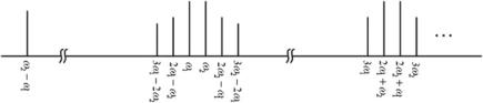
It can be seen that after the dual-tone signal enters the nonlinear equipment, many parasitic products with different frequencies are generated. The frequency spectrum is shown in Fig. 5.73 [59].
If ω1 and ω2 are close to each other, all the even-order products will be far away from ω1 and ω2, such that they are easy to be filtered out from the output spectrum. The odd-order products, on the other hand, are likely to fall into the passband or near
218 |
5 Critical Techniques of Quantitative System-Level EMC Design |
the passband. The third-order output signal is one of them, and it has the greatest effect on normal signals since the order is low and the power is strong.
Let PC W be the output power of the signal at ω1, and we can perform the approximate calculation ignoring the terms with small amplitude and with order higher than three. From Eq. (5.196), we can get
PC W |
1 |
|
2 a12 V02/Z0 |
(5.197) |
where Z0 is the impedance of the receiver RF system and can be set to 50 . Similarly, let PO I M3 be the signal output power at the third-order intermodulation
frequency ω ( ω 2ω1 − ω2). According to (5.196), we have
|
1 |
3 |
2 |
|
||
PO I M3 |
a3 V03 /Z0 |
(5.198) |
||||
|
|
|
||||
2 |
4 |
|||||
When PC W and PO I M3 are equal at the TOI point, the output signal voltage is
VO I M3 |
4a1 |
(5.199) |
3a3 |
When the output power PO I P3 at the intercept point is equal to the linear response , we have the following equation according to (5.197) and (5.198):
|
2a3 |
|
|
PO I P3 PC W V0 VO I M3 |
1 |
/Z0 |
(5.200) |
3a3 |
Combining (5.197), (5.198), and (5.200), we can get the constraint among PO I M3,
PC W , and PO I P3 as |
|
|
|
|
|
|
|
|
|
|
|
|
|
|
|
9a2 V 6 |
|
a6 V 6 |
4a6 |
|
(PC W )3 |
|
|||||||
|
3 |
0 |
1 |
0 |
|
1 |
|
|
|
|
|
|||
PO I M3 |
|
|
/Z0 |
|
/ |
|
|
|
|
|
|
(5.201) |
||
32 |
|
8Z0 |
9a32 Z0 |
(PO I P3)2 |
||||||||||
Then, we can obtain the constraint among VO I M3, PC W , and PO I P3 as |
|
|||||||||||||
|
|
|
|
|
|
|
|
|
|
|
||||
|
|
|
|
|
|
|
|
|
(PC W )3 Z0 |
|
|
|||
VO I M3 |
|
PO I M3 Z0 |
(5.202) |
|||||||||||
|
|
PO I P3 |
||||||||||||
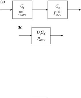
Assume G1 and PO(1I)P3 are the power gain of the first stage and the output power of the first-stage TOI point, respectively; and assume G2 and PO(2I)P3 are the power gain of the second stage and the output power of the second-stage TOI point, as shown in Fig. 5.74. From (5.201), we can get the third-order distortion power at the output of the first stages
5.4 EMC Simulation Method |
219 |
Fig. 5.74 Example of a TOI point equivalent to the cascade system. a Two cascade networks.
b Equivalent network
|
P(1) |
3 |
|
|
|
|
|
PO(1)I M3 |
C W |
|
(5.203) |
|
|||
P(1) 2 |
|||
|
O I P3 |
|
|
where PC(1W) is the power of a single interference continuous wave output for the first stage.
The voltage associated with the third-order distortion power at the output of the first stage is
|
|
|
P |
(1) |
3 |
Z0 |
|
|
|
|
|
||||
|
|
|
|
|
|||
VO(1)I M3 PO(1)I M3 Z0 |
C W |
|
|
(5.204) |
|||
P |
(1) |
|
|
||||
|
|
|
O I P3 |
|
|
||
In a cascaded system, the intermodulation products are deterministic signals (coherent signals), which cannot simply be a sum of power, but needs to be handled in voltage. These voltages are phase dependent, and there are phase delays at all levels, which may cause local cancelation. Here, in order to consider the worstcase interference signal strength, it is assumed that all signals do not have in-phase
|
|
|
|
|
|
|
|
|
|
|
|
|
|
|
|
|
|
|
|
|
|
|
(2) |
of the |
||
cancelation. The third-order intermodulation distortion voltage output VO I M3 |
||||||||||||||||||||||||||
second stage is the third-order intermodulation distortion voltage output V |
(1) |
of the |
||||||||||||||||||||||||
first stage multiplied by the voltage gain √ |
|
|
|
|
|
|
|
|
|
I M3 |
|
|
||||||||||||||
G2 |
|
of the second stage and the distortion |
||||||||||||||||||||||||
|
|
|
P(2) |
3 |
Z0 |
|
|
|
|
|
|
|
|
|
|
|
|
|
|
|
|
|
|
|||
|
|
|
|
|
|
|
|
|
|
|
|
|
|
|
|
|
|
|
|
|
||||||
voltage |
|
|
C W |
|
|
generated by the second stage, that is |
|
|
|
|
|
|
|
|
||||||||||||
|
P(2) |
|
|
|
|
|
|
|
|
|
|
|||||||||||||||
|
|
|
O I P3 |
|
|
|
|
|
|
|
|
|
|
|
|
|
|
|
|
|
|
|
|
|
|
|
|
|
|
|
|
|
|
|
|
|
|
|
|
|
|
|
|
|
|
|
|
|
|
|
|
|
|
|
|
|
|
|
|
|
|
|
|
P(2) |
3 |
|
|
|
|
|
|
G2 P(1) |
3 |
|
|
|
P(2) |
3 |
|
|
|
|
|
|
|
|
|
|
|
|
|
Z0 |
|
|
Z0 |
Z0 |
|||||||||||
VO(2)I M3 |
VO(1)I M3 |
|
+ |
|
C W |
|
|
|
|
|
C W |
|
+ |
|
C W |
|
|
|
||||||||
G2 |
|
|
|
|
|
|
|
|
|
|
|
|
|
|||||||||||||
|
P(2) |
|
|
|
|
P(1) |
|
|
P(2) |
|
|
|
||||||||||||||
|
|
|
|
|
|
|
|
|
|
O I P3 |
|
|
|
|
|
|
O I P3 |
|
|
|
|
O I P3 |
|
|
||
|
|
|
|
|
|
|
|
|
|
|
|
|
|
|
|
|
|
|
|
|
|
|
|
(5.205) |
||
where PC(2W) is the power of a single interference continuous wave output for the second stage; since PC(2W) G2 PC(1W) , then

220 5 Critical Techniques of Quantitative System-Level EMC Design
|
VO(2)I M3 |
|
|
1 |
|
+ |
1 |
|
|
|
|
PC(2)W |
3 |
|
(5.206) |
|||||
|
|
|
|
|
|
|
|
|
|
|
Z0 |
|||||||||
|
|
G2 P(1) |
|
P(2) |
|
|
|
|||||||||||||
|
|
|
|
|
|
O I P3 |
O I P3 |
|
|
|
|
|
|
|||||||
The output distortion power is |
|
|
|
|
|
|
|
|
|
|
|
|
|
|
|
|||||
|
VO(2)I M3 |
2 |
|
|
|
|
|
|
|
|
|
|
|
|
|
|
|
3 |
|
|
|
|
|
1 |
|
|
|
|
1 |
|
|
2 |
3 |
|
PC(2)W |
|
|||||
PO(2)I M3 |
|
|
|
|
|
|
+ |
|
|
|
|
|
PC(2)W |
|
|
(5.207) |
||||
Z0 |
|
G2 P |
(1) |
P(2) |
|
|
|
( PO I P3)2 |
||||||||||||
|
|
|
|
|
O I P3 |
|
|
|
O I P3 |
|
|
|
|
|
|
|
|
|||
Then, the TOI point of the cascade system is |
|
|
|
|
|
|
|
|
||||||||||||
|
|
|
PO I P3 |
|
|
1 |
|
|
+ |
|
|
1 |
|
−1 |
|
|
(5.208) |
|||
|
|
|
|
|
|
|
|
|
|
|
|
|
||||||||
|
|
|
|
|
|
|
|
|
|
|
|
|||||||||
|
|
|
|
G2 P(1) |
|
P |
(2) |
|
|
|
|
|||||||||
|
|
|
|
|
|
|
|
|
O I P3 |
|
O I P3 |
|
|
|
||||||
By analogy, the constraint of the total distortion voltage of the receiver RF system and the TOI points at each level can be written as
|
|
|
|
|
|
P(2) |
3 Z0 |
|
|
|
|
P(N −1) 3 Z0 |
|
|
|
P |
(N ) 3 Z0 |
||||||
|
|
|
|
|
|
C W |
|
|
|
|
|
|
|
C W |
|
|
|
|
|
|
C W |
||
VO I M3 |
VO(1)I M3 G2 + |
|
|
|
G3 + · · · + |
|
|
|
G N + |
||||||||||||||
P(2) |
|
|
|
|
|
P(N −1) |
|
|
|
P |
(N ) |
|
|||||||||||
|
|
|
|
|
|
O I P3 |
|
|
|
|
|
O I P3 |
|
|
|
|
|
|
O I P3 |
||||
|
|
|
|
|
|
|
|
|
|
|
|
|
|
|
|
|
|
|
|
|
|
(5.209) |
|
The corresponding output power of the cascade TOI point is |
|
|
|
|
|
|
|||||||||||||||||
PO I P3 |
|
1 |
|
+ |
|
1 |
|
|
+ · · · + |
1 |
|
|
−1 |
(5.210) |
|||||||||
|
|
|
|
|
|
|
|
|
|||||||||||||||
|
|
|
|
|
|
|
|
|
|
|
|
|
|
||||||||||
|
|
|
|
(1) |
|
(2) |
|
|
(N ) |
|
|
|
|
||||||||||
|
|
|
G N · · · G2 PO I P3 |
|
G N · · · G3 PO I P3 |
PO I P3 |
|
|
|
|
|
|
|||||||||||
where P(i) |
|
is the output TOI point power of the i-th sub-circuit; P |
(i) |
is the output |
|||||||||||||||||||
O I P3 |
|
|
|
|
|
|
|
|
|
|
|
|
|
|
|
C W |
|
|
|
|
|||
power of a single interfering continuous wave through the i-th sub-circuit, and it can be expressed as
PC(iW) Gi PC(iW−1) (i 2, 3, . . . , N ) |
(5.211) |
Usually, the passband of the filter in the prestage circuit of the superheterodyne receiver RF system is relatively wide. Assuming that both interference continuous waves fall within the filter passband, then there is no attenuation of the desired signal and the third-order intermodulation signal. The passband of the IF filter is narrow; thus, there will be attenuation Li (Li < 1) to the interference continuous wave. The attenuation is introduced to correct the cascade equation of the TOI point.
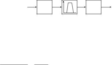
Figure 5.75 is a cascade block diagram considering the selectivity of the filter in the RF system. Due to the selective suppression of the continuous wave interference signal by the filter module, Eq. (5.211) can be modified to
5.4 EMC Simulation Method
Fig. 5.75 Cascade block diagram considering filter selectivity in RF systems
221
G1 |
L2 |
G2 |
|
||
P(1) |
|
P(2) |
OIP3 |
|
OIP3 |
PC(iW) Gi Li PC(iW−1) (i 2, 3, . . . , N )
where Li is the attenuation of the continuous wave interference signals (the frequencies are ω1 and ω2) from the i-th filter module.
Here, when the module in the middle of Fig. 5.75 contains multiple filters, it will be unified to an attenuation value L2.
Taking into account the module that contains the frequency selection characteristics, we can derive the following equation from (5.205) as
|
|
P(2) |
3 |
|
|
P(2) |
3 |
|
|
|
|
|
|
|
|
|
|
|
|
|
|
|
G2 |
G2 L2 Z0 |
|
|
Z0 |
|
|
1 |
|
|
|
|
1 |
|
|
|
|||||
|
|
|
|
|
|
|
|
|
3 |
|
|||||||||||
|
|
C W |
|
|
|
C W |
|
|
|
|
|
|
|
|
|
|
|||||
VO(2)I M3 |
|
|
|
+ |
|
|
|
|
|
|
|
|
|
|
+ |
|
|
|
PC(2)W Z0 |
||
|
P |
(1) |
P(2) |
|
|
G |
2 P(1) |
|
(L2)3/ 2 |
P |
(2) |
||||||||||
|
|
O I P3 |
|
|
O I P3 |
|
|
|
O I P3 |
|
|
|
O I P3 |
(5.212) |
|||||||
|
|
|
|
|
|
|
|
|
|
|
|
|
|
|
|
|
|
|
|||
The TOI point of the cascade system is |
|
|
|
|
|
|
|
|
|
|
|
|
|||||||||
|
|
|
PO I P3 |
|
|
|
1 |
|
|
|
+ |
|
|
1 |
−1 |
|
|
(5.213) |
|||
|
|
|
|
|
|
|
|
|
|
|
|
|
|
|
|||||||
|
|
|
|
|
|
|
|
|
|
|
|
|
|||||||||
|
|
|
|
G2 P(1) |
|
(L2)3/ 2 |
P |
(2) |
|
|
|
|
|||||||||
|
|
|
|
|
|
O I P3 |
|
|
|
|
O I P3 |
|
|
|
|
|
|||||
Similarly, the corrected output power of the TOI point of the receiving equipment
is
|
1 |
|
|
|
1 |
|
|
1 |
−1 |
|
PO I P3 |
|
|
|
+ |
|
|
|
+ · · · + |
|
|
(1) |
(L N · · · L2) |
3/ 2 |
(2) |
(L N · · · L3) |
3/ 2 |
(N ) |
|
|||
|
G N · · · G2 PO I P3 |
|
|
G N · · · G3 PO I P3 |
|
|
PO I P3 |
|
||
(5.214)
It can be seen from (5.214) that the filtering module will reduce the output power of the third-order intermodulation signal; when a filter with better selectivity is used in the latter stage (Li << 1), the total output power of the TOI point of the receiving equipment is basically determined by the preceding stage.
(2)Method for allocating third-order intermodulation distortion parameters in system modeling
Whether to design a RF system of the transmitting/receiving equipment or to simulate and evaluate the system communication quality, the overall parameters provided by the RF system are signal-to-noise ratio (SNR), total noise figure (NF), bandwidth, dynamic range, gain, etc. The third-order intermodulation distortion parameters of the sub-circuit module are not included. Third-order intermodulation interference signals, which have a severe impact on normal signals, can often be generated and amplified in transmitting equipment and cause interference to other communication
222 |
|
|
|
|
|
|
5 Critical Techniques of Quantitative System-Level EMC Design |
|||||||||||||||||||||
|
|
|
|
|
|
|
|
|
|
|
|
|
|
|
|
|
|
|
|
|
|
|
|
|
|
|
|
|
|
|
|
|
|
|
|
|
|
|
|
|
|
|
|
|
|
|
|
|
|
|
|
|
|
|
|
|
|
|
|
|
|
|
|
|
|
|
|
|
|
|
|
|
|
|
|
|
|
|
|
|
|
|
|
|
|
|
|
|
|
|
|
|
|
|
|
|
|
|
|
|
|
|
|
|
|
|
|
|
|
|
|
|
|
|
|
Fig. 5.76 Diagram of the ultrashort wave radio receiver from the case
platforms. If the design specifications of the receiving equipment do not include clear determinations of the third-order intermodulation distortion parameters, parasitic responses will be easily caused and the dynamic range will be greatly reduced. The accurate design of the third-order intermodulation distortion parameters of the subcircuits in the RF system of the receiver can ensure that the receiver does not cause the degradation of the sensitivity and the deterioration of the communication quality due to the third-order intermodulation distortion signal being too large. Therefore, the third-order intermodulation distortion parameters of each sub-circuit module need to be reasonably allocated according to the overall performance indicator of the RF system.
We use an ultrashort wave radio as an example to describe the stepwise allocation of the third-order intermodulation distortion parameters of the receiving equipment from the top-level requirements to the sub-layers. The principle diagram is shown in Fig. 5.76. The RF system includes a front-end low-noise amplifier (LNA), the filter A, the first mixer, the first IF filter, the first IF amplifier, the second mixer, the second IF filter, the second IF amplifier, and the compensation amplifier B. The receiving equipment parameters are set as: The receiving frequency is 86 MHz, the total noise figure is 4.6 dB, the IF bandwidth is 68 kHz, and the receiving sensitivity is −93 dBm.
When multiple communication systems operate at the same time, the power of the signal entering the receiving system emitted from the adjacent channels is −30 dBm. During the analysis and design of the receiver, it is required that the maximum output power of the third-order intermodulation signal of the −30 dBm dual-tone signal through the receiving equipment is no larger than the maximum output noise power generated by the circuit within the system.
The two frequencies selected for the adjacent channel transmission signal are ω1 85.475 MHz and ω2 84.925 MHz, and the frequency of the third-order intermodulation distortion signal falling within the reception passband is ω 2ω1 − ω2 86.025 MHz. The attenuation of the two frequencies by filter A and the first IF filter is neglected. The sub-circuit modules that affect the power of the third-order intermodulation signal include the front-end LNA, the first mixer, the first IF amplifier, the second mixer, the second IF amplifier, the second IF filtering, and the compensation amplifier B.
The sensitivity of the receiver is −93 dBm. After the IF output, a high signal level is achieved. The total gain of this receiver RF system is 87 dB. The gain and noise figure of each module are shown in Table 5.15.
The total noise figure of the receiver is [19]
5.4 EMC Simulation Method
Table 5.15 Gain and noise figure of the modules in the receiving system
|
|
223 |
|
|
|
Sub-module |
Gain G (dB) |
Noise figure F (dB) |
|
|
|
Front-end LNA |
8 |
2.8 |
module |
|
|
|
|
|
First mixing module |
6 |
7 |
|
|
|
First IF amplifier |
10 |
9.5 |
module |
|
|
|
|
|
Second mixing |
6 |
7 |
module |
|
|
|
|
|
Second IF amplifier |
25 |
9.5 |
module |
|
|
|
|
|
Compensation |
32 |
8 |
amplifier module |
|
|
|
|
|
F |
|
F + |
F2 − 1 |
+ |
F3 − 1 |
+ |
· · · |
+ |
F6 − 1 |
(5.215) |
|
|
G1 G2 G3 G4 G5 |
||||||||
|
1 |
G1 |
G1 G2 |
|
|
|||||
where F is the ground truth of the total noise figure of the receiver RF system. The relationship between F and the figure from Table 5.15 is F(dB) 10 log10 F (ground truth).
According to Table 5.15, the total noise figure is 4.6 dB, the total gain is 87 dB,
and the noise power output from the receiver RF system is |
|
No Gk B [TA + (F − 1)To] |
(5.216) |
where G is the total gain of the receiving RF system; k is the Boltzmann constant (1.38 × 10⁻²³ J K ); B is the IF bandwidth of the receiver RF system; TA is the equivalent noise temperature fed to the receiver antenna; F is the total noise figure of the receiver RF system; T0 is the temperature (T0 290 K). Substituting the above value into (5.216),
No 108.7 × 1.38 × 10−23 × 68 × 103 × [290 + (100.46 − 1) × 290] 3.93 × 10⁻⁷W
i.e., −34.05 dBm.
In order to suppress the influence of the transmitting signal from the adjacent channel to the receiver, two continuous waves at 84.925 and 85.475 MHz are used as the interference signal, to calculate the third-order intermodulation distortion that falls into the receiving passband after N0 passes through the receiver RF system. It is required that the power intensity at the IF output end is no greater than the maximum output noise power generated by the circuit within the system; i.e., there is no spurious response. Therefore, the maximum output power of the total thirdorder intermodulation distortion signal allowed by the receiving RF system is −34.05 dBm. The converted voltage is VO I M3 4.43 × 10⁻³ V. Figure 5.77 is a behavioral simulation circuit model for an RF front-end system of an ultrashort wave receiver.
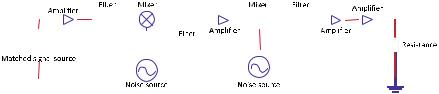
224 |
|
|
|
|
|
|
|
|
5 Critical Techniques of Quantitative System-Level EMC Design |
|||||||||||||||||||||||||
|
|
|
|
|
|
|
|
|
|
|
|
|
|
|
|
|
|
|
|
|
|
|
|
|
|
|
|
|
|
|
|
|
|
|
|
|
|
|
|
|
|
|
|
|
|
|
|
|
|
|
|
|
|
|
|
|
|
|
|
|
|
|
|
|
|
|
|
|
|
|
|
|
|
|
|
|
|
|
|
|
|
|
|
|
|
|
|
|
|
|
|
|
|
|
|
|
|
|
|
|
|
|
|
|
|
|
|
|
|
|
|
|
|
|
|
|
|
|
|
|
|
|
|
|
|
|
|
|
|
|
|
|
|
|
|
|
|
|
|
|
|
|
|
|
|
|
|
|
|
|
|
|
|
|
|
|
|
|
|
|
|
|
|
|
|
|
|
|
|
|
|
|
|
|
|
|
|
|
|
|
|
|
|
|
|
|
|
|
|
|
|
|
|
|
|
|
|
|
|
|
|
|
|
|
|
|
|
|
|
|
|
|
|
|
|
|
|
|
|
|
|
|
|
|
|
|
|
|
|
|
|
|
|
|
|
|
|
|
|
|
|
|
|
|
|
|
|
|
|
|
|
|
|
|
|
|
|
|
|
|
|
|
|
|
|
|
|
|
|
|
|
|
|
|
|
|
|
|
|
Fig. 5.77 Behavioral simulation model of the ultrashort wave receiving radio RF front end
Table 5.16 Output power of the TOI point and output voltage/power of the third-order intermodulation signal at each level of the receiving system
Sub-module |
Output TOI point |
Third-order |
Third-order |
|
power (dBm) |
intermodulation |
intermodulation |
|
|
signal voltage (V) |
signal power (dBm) |
|
|
|
|
Front-end LNA module |
30 |
1.121 × 10⁻⁷ |
−126.00 |
First mixing module |
35 |
2.815 × 10⁻⁷ |
−112.92 |
First IF amplifier module |
50 |
1.879 × 10⁻⁶ |
−101.51 |
Second mixing module |
55 |
4.456 × 10⁻⁶ |
−94.01 |
Second IF amplifier |
40 |
7.924 × 10⁻⁵ |
−69.01 |
module |
|
|
|
Compensation amplifier |
40 |
3.155 × 10⁻³ |
−37.00 |
module |
|
|
|
Considering the worst-case total third-order intermodulation distortion voltage, the third-order intermodulation distortion parameters are assigned to the modules with nonlinear characteristics inside the RF system circuit of the receiver according to (5.212). The power of the third-order intermodulation signal generated by each module is being strictly controlled as shown in Table 5.16.
It can be seen from Table 5.16 that the second IF filter suppresses the power of the two continuous wave signals by 75 dB, which is used to improve the TOI point of the subsequent stage. The output power of the TOI point from the second IF amplification can be adjusted to a smaller value. According to the assigned value, the calculated total third-order intermodulation distortion voltage is VO I M3 3.155 × 10⁻³ V (less than VO I M3 4.43 × 10⁻³ V), which satisfies the requirement. It means that the generated third-order intermodulation distortion signal will not affect the normal communication of the receiver.
It is worth mentioning that although there is more than one method of allocating the third-order intermodulation distortion parameters, it is necessary to strictly follow the modified TOI point cascade equations to control the voltage of control signals step by step in the simulation model, so that the overall indicator will meet the requirements. Using the overall performance indicator, we can analyze the reasonable third-order intermodulation distortion parameters of all internal sub-circuits, such that with limited parameters available, we can guarantee the parasitic-response-free dynamic range of the receiver.
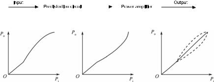
5.4 EMC Simulation Method |
225 |
||||
|
|
|
|
|
|
|
|
|
|
|
|
|
|
|
|
|
|
(a) |
(b) |
(c) |
Fig. 5.78 Block diagram of the predistortion techniques and linearization. a Amplifier input/output transfer characteristics; b input/output transfer characteristics of the predistortion circuit; and c overall input/output transfer characteristics
(3) Analog predistortion circuits to suppress the low-order intermodulation
Last section focuses on the allocation of the third-order intermodulation distortion parameters of the RF system of the communication equipment using the overall requirements during the EMC design of the receiving system. The strength of the interfering signal gets controlled after entering the system and meets the system requirements. From the transmitting system point of view, this section provides a feasible solution to improve EMC, and a circuit that suppresses the third-order and fifthorder intermodulation distortions. The effectiveness of the circuit is then verified.
High-power signal radiation in the transmitting system is accompanied by a strong spurious signal group. The major source of these spurious signals is power amplifiers which usually operate in the nonlinear region to improve the efficiency [60]. There are many linearization techniques, such as feedforward, negative feedback, and predistortion to deal with the nonlinear problems in power amplifiers. Negative feedback technique has a simple circuit structure and is low cost, but it is instable. Feedforward technique can provide good linearity, but the complex and expensive analog equipment it uses are difficult to control. Thus, the predistortion technique is a low-cost technique which is also easy to model in simulation software [61].
The basic idea of the predistortion technique is to insert a piece of nonlinear equipment in front of the RF power amplifier so that the power amplifier’s transmission characteristic is close to linear and the out-of-band diffusion is reduced. Its block diagram and transmission characteristics are shown in Fig. 5.78. The transform characteristics of the predistortion circuit are used to compensate for the nonlinear characteristics of the main power amplifier, such that the intermodulation distortion can be canceled and the nonlinearity of the power amplifier gets improved. The advantage of predistortion technology is that there is no stability problem and the price is low. Several carefully selected components are packaged into a single module and connected between the signal source and the power amplifier to form a predistortion linear power amplifier [62].
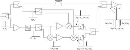
226 |
|
5 Critical Techniques of Quantitative System-Level EMC Design |
||
Subdivider |
Path 1 |
|
Delay |
Combiner Amplifier |
|
|
|||
|
|
|
|
|
|
|
Subdivider |
|
Output |
|
|
|
|
|
Input |
|
|
|
|
Subdivider |
|
|
|
|
Amplifier |
Filter |
Subdivider |
Amplifier |
|
|
|
|||
Path 2 |
|
|
Amplifier Mixer |
|
|
|
|
|
Combiner |
|
|
Mixer |
Mixer |
|
Fig. 5.79 Implementation block diagram of the predistortion circuit
The actual implementation of the analog predistortion circuit is shown in Fig. 5.79. The input dual-tone signal (ω1, ω2) is split by the power splitter into the fundamental and intermodulation distortion signals to generate two paths: linear path 1 and nonlinear path 2. The input signal in path 1 is delayed, and a nonlinear intermodulation distortion signal is generated in path 2, which enters the power amplifier together with the original dual-tone signal. Let the two signals be A1 cos(ω1t) and A2 cos(ω2t), and the signal of the input end of the predistortion circuit is:
x(t) A1 cos(ω1t) + A2 cos(ω2t) |
(5.217) |
After passing through the first amplifier and filter in path 2, a second-order component ω2 − ω1 is obtained, and the signal strength is weak. After that, ω2 − ω1 is frequency doubled to generate component 2(ω2 − ω1). The components 2(ω2 − ω1) and ω2 − ω1 are then mixed with the fundamental waves ω1 and ω2, respectively, to generate 2ω2 − ω1, 2ω1 − ω2, 3ω2 − 2ω1, and 3ω1 − 2ω2. Finally, after amplitude and phase shift adjustment, the weak even-order signals are ignored. The output signal of path 2 is
b(t) A11 cos(2ω1t − ω2t + ϕ11) + A22 cos(2ω2t − ω1t + ϕ22) + A33 cos(3ω1t − 2ω2t + ϕ33)
+ A44 cos(3ω2t − 2ω1t + ϕ44) |
(5.218) |
where A11, A22, A33, and A44 are the voltages for each component; ϕ11, ϕ22, ϕ33, and ϕ44 are the corresponding phases.
The generated phase-inverted signal is used to cancel the low-order intermodulation distortion signal of the power amplifier. The actual input signal of the power amplifier is x(t) + b(t).
Here, we provide an example in which a power amplifier with the predistortion circuits is designed, then tests are performed using Agilent ADS circuit analysis software, and finally the behavioral simulation method is used to implement the predistortion circuit and verify its effectiveness.
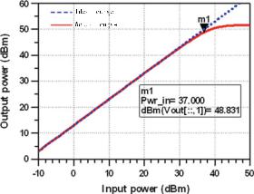
5.4 EMC Simulation Method |
227 |
Fig. 5.80 Input and output characteristics of the power amplifier harmonic balance simulation
The power amplifier has a gain of 13 dB, and a harmonic balance simulator is used to calculate the behavioral model of the power amplifier. The input and output transfer characteristics are shown in Fig. 5.80. In the figure, m1 is close to the 1 dB compression point. The signal power of m1 is 37 dBm. The amplifier operates in the nonlinear region, and spurious components appear in the output signal. When there are multiple carrier signals in the input, the odd-order intermodulation interference signal is close to the normal signal, and it will be difficult to filter out.
In odd-order intermodulation signals, the low-order signal is strong. For the generated third-order and fifth-order intermodulation interference, we can add a simple predistortion circuit before the power amplifier. Figure 5.81 is a behavioral simulation model built according to the process in Fig. 5.79. Suppose the frequencies ω1 and ω2 of the dual-tone signal entering the power amplifier are 836 MHz and 842 MHz, respectively, and the second-order component with a frequency of 6 MHz (ω2 − ω1) is obtained in path 2 through a low-pass filter. Actually, the closer ω1 and ω2 are, the smaller ω2 − ω1 is, therefore, the easier it is to implement the low-frequency filter circuit design; the second-order component is then multiplied to obtain the 6 and 12 MHz signals simultaneously, and then the mixing, AM, and PM procedures are performed to the signal to obtain the third-order intermodulation component signals, of which the frequencies are 830 MHz (2ω1 − ω2) and 848 MHz (2ω1 − ω2). In addition, the fifth-order intermodulation component signals, of which the frequencies are 824 MHz (3ω1 − 2ω2) and 854 MHz (3ω1 − 2ω2), are generated. The signals generated in path 2 will enter the main power amplifier together with the original input signal to suppress the signal strength of the total output third-order and fifth-order intermodulation.
After the dual-tone signal in path 1 enters the power amplifier, the third-order and fifth-order intermodulation products with strong power are generated in addition to the main frequency. The intermodulation products generated in path 2 will output a phase-inverted signal waveform through the power amplifier; in other words, the waveform has a phase difference of approximately 180 degree from the intermodu-
228 |
|
|
5 Critical Techniques of Quantitative System-Level EMC Design |
|||
|
Amplifier |
Filter |
Frequency |
Filter |
Amplifier |
Harmonic Simulation |
|
|
|
Synthesizer |
|
|
|
Power Divider |
|
|
|
Mixer |
|
|
|
|
|
|
|
|
|
|
|
|
Combiner |
|
|
|
Matched Signal Source |
|
|
|
DC Power |
|
|
|
|
|
|
|
|
|
|
|
|
|
|
|
Matched Load |
|
Power Divider |
|
Delayer |
Combiner Amplifier |
||
|
|
|
|
|||
Fig. 5.81 Behavioral simulation model of the predistortion circuit |
|
|||||
(a) |
|
|
|
|
(b) |
|
|
Generative Predistortion Intermodulation Signal |
generated predistortion |
||||
|
|
|
|
|
|
inter-modulation signal |
|
|
|
|
|
|
treble inter-modulation |
|
|
|
|
|
|
signal |
Power Divider |
Filter |
Filter |
Amplifier |
|
Matched |
|
|
|
|
|
|
|
|
|
|
|
|
|
load |
|
|
|
|
Treble Intermodulation Signal |
|
||
|
Amplifier |
Power Divider |
|
|
|
|
Matched Signal |
|
Filter |
|
Filter |
|
|
|
|
|
|
|
||
Source |
|
|
|
|
|
|
|
|
|
Matched Load |
|
|
|
Fig. 5.82 |
Two-part third-order intermodulation signal simulation model and signal waveforms. |
|||||
a Third-order intermodulation signal extraction from path 1 and path 2 and b two third-order intermodulation signal waveforms of final output
lation signal generated in path 1. Here, we choose to observe the waveform of the third-order component 2ω1 − ω2, which includes two parts: One is the third-order intermodulation signal which is generated by the predistortion and then amplified; the other is the third-order intermodulation signal generated by the main power amplifier. The simulation circuit generating the two parts of the signal is shown in Fig. 5.82a: Using the ideal filter, the intermodulation signal with a frequency of 830 MHz from the mixed signals before entering the power amplifier is obtained as shown in Fig. 5.81, and the output waveform is given after the power amplifier; the dual-tone signal is directly used to enter the power amplifier, and an ideal filter is used to obtain an intermodulation signal with a frequency only of 830 MHz. The waveforms of the two third-order intermodulation signals are shown in Fig. 5.82b. It can be seen that the phase difference between the two is about 180°.
The output spectrum of the power amplifier before and after the predistortion improvement is shown in Fig. 5.83. It can be seen that the third-order intermodulation can be improved at least 15 dB and the fifth-order intermodulation can be improved 9 dB.
The power output capability and linear performance of the RF power amplifier directly affect the quality of the wireless communication. In the design process, the
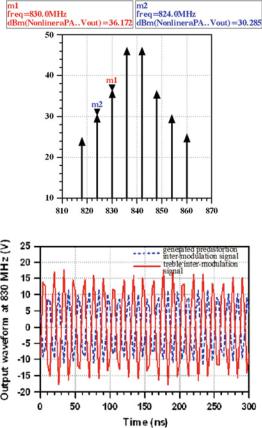
5.4 EMC Simulation Method |
229 |
|
Fig. 5.83 Output spectrum |
(a) |
|
of the power amplifier before |
|
|
and after using predistortion |
|
|
techniques. a Output |
|
|
spectrum before |
predistortion/dBmbeforePower |
|
predistortion and b output |
||
|
||
spectrum after predistortion |
|
|
|
Frequency/MHz |
|
|
(b) |
predistortion circuit can be introduced if needed. Several components are selected to form a single module, connecting the low-order intermodulation output before being connected to the main power amplifier. In addition, during the analysis of the actual system EMC, the emission system that does not meet the regulation requirements after testing needs to suppress the intermodulation interference signals using necessary approaches. It is rare for existing equipment to be required to undergo massive troubleshooting. In order to meet the actual requirements of the system, we only need to build a predistortion circuit in front of the nonlinear amplifier in the predistortion model to reduce the strong third-order and fifth-order intermodulation signal interference caused by the nonlinear characteristics. The implementation is simple and effective.
230 |
5 Critical Techniques of Quantitative System-Level EMC Design |
5.4.3Identification of Electromagnetic Emission Elements Based on Gray Model (Case 3)
The ultimate goal of the EMC study of electronic equipment is to make the equipment or system work properly in its electromagnetic environment without producing intolerable EMI to other equipment in the environment. In this section, we propose a method to analyze the EMC test spectrum [63], introduce the important electromagnetic emission elements, and identify potential causes of interference. The methods can be used to guide the equipment troubleshooting and quantitative design in early stage.
The characteristics of the electromagnetic spectrum obtained from test can be summarized as follows:
(1)Inherit attributes. As a causal system, the characteristics of the interference source can be extracted from the electromagnetic emission spectrum of the EUT.
(2)Discreteness. Although the electromagnetic emission of the equipment is continuous, the frequency spectrum measured by the EMI receiver is the emission field strength obtained at specific frequencies with a certain sampling interval.
(3)Complexity. Due to equipment nonlinearity, cable cross talk, case shielding, test environment, and other factors, the measured spectrum is extremely complicated, and there are interferences in the frequency range from several kilohertz to even megahertz.
(4)Observed spectrum. Electromagnetic emission spectrum is often as wide as hundreds of octaves, but a considerable part of the spectrum is the “observed spectrum” generated by the basic interference elements under nonlinear effects.
Since the spectrum obtained from equipment testing can always reflect the characteristics of the equipment’s internal sources, studying the characteristics of the spectrum is very important for understanding the equipment’s EMC. However, due to the complexity of the spectrum, the research process needs to be simplified and starts from the most typical spectrum. Considering the discrete nature of the frequency points, we first need to decide a method to analyze the discrete data.
From the analysis of the circuit mechanism, we know that the harmonics, as an interference element, is very important in electromagnetic spectrum. To better understand the test data, it is highly necessary to accurately extract the characteristics of the harmonics.
The goal of electromagnetic spectrum processing in view of harmonics is to extract the electromagnetic characteristics of the harmonic interference elements from the measured interference spectrum. Harmonic interference extraction process is shown in Fig. 5.84. First of all, the spectrum obtained from the test is preprocessed; that is, the overall trend component in the spectrum is extracted; then, the total
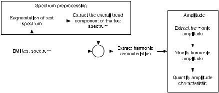
5.4 EMC Simulation Method |
231 |
||||||||||||||
|
|
|
|
|
|
|
|
|
|
|
|
|
|
|
|
|
|
|
|
|
|
|
|
|
|
|
|
|
|
|
|
|
|
|
|
|
|
|
|
|
|
|
|
|
|
|
|
|
|
|
|
|
|
|
|
|
|
|
|
|
|
|
|
|
|
|
|
|
|
|
|
|
|
|
|
|
|
|
|
|
|
|
|
|
|
|
|
|
|
|
|
|
|
|
|
|
|
|
|
|
|
|
|
|
|
|
|
|
|
|
|
|
|
|
|
|
|
|
|
|
|
|
|
|
|
|
|
|
|
|
|
|
|
|
|
|
|
|
|
|
|
|
|
|
|
|
|
|
|
|
|
|
|
|
|
|
|
|
|
|
|
|
|
|
|
|
|
|
|
|
|
|
|
|
|
|
|
|
|
|
|
|
|
|
|
|
|
|
|
|
|
|
|
|
|
|
|
|
|
|
|
|
|
|
|
|
|
Fig. 5.84 Extraction process of the harmonic interference
trend component is subtracted from the total interference spectrum to extract the frequency of the harmonic component in the remaining spectrum; next, in accordance with the harmonic frequency, amplitude characteristics of the harmonic frequency are extracted; finally, we can get an overall understanding of the electromagnetic properties of the harmonics.
1. Spectral data preprocessing based on the gray model
First of all, the test data is preprocessed, and the gradual change components in the emission spectrum are extracted and eliminated. Then, we analyze the characteristics of the components with great impact on the spectrum.
We have tried to apply the gray system model to the spectrum sequence modeling in EMC based on our long-term study of the model. The GM (1, 1) model in the gray system theory is used to model the overall trend component.
The meanings of the symbol GM (1, 1) are as follows:
G |
M |
(1, |
1) |
↑ |
↑ |
↑ |
↑ |
Gray model 1st order function 1 variable
In order to simplify the analysis process, the spectrum obtained from the test is compared with the limit value of the EMI emission before the spectrum analysis, and the part beyond the regulation is studied.
(1) Spectrum segmentation
Assuming that the spectrum data of the EMI test is X {x(1), x(2), · · · , x(n)}, the mean sequence of each small segment is calculated using (5.219), i.e.,
232 |
5 Critical Techniques of Quantitative System-Level EMC Design |
|||
|
S(1 + (K − 1)l1 : kl1) |
kl1 |
(k 1, 2, . . . , n l1) |
|
|
X(i)/ l1 |
(5.219) |
||
i 1
The length of the selected segment, denoted as l1, can be adjusted according to the length of the test sequence.
Then, we can find the segment points in the generated ladder-shaped curves and extract the segment points in the analysis spectrum as x(s1), x(s2), · · · , x(sm ). The spectrum is thus divided into (sm + 1) segments.
(2) Overall trend component modeling
The test data usually has a certain overall trend, which reflects the superposition of the equipment’s broadband interference and the gradual change components in the environment level. The contribution of this component to the spectrum is not significant. The overall trend component of the broadband needs to be eliminated to extract other forms of interference.
Before the establishment of the overall trend component, the sequence to be
modeled must be cumulatively generated first. |
|
|
|
|
|
|
|
|
||
The original modeling sequence is X |
(0) |
(x(0) |
(1), |
x(0)(2), . . . , x(0)(n)). After |
||||||
|
(1) |
|
(1) |
(1), x |
(1) |
(2), . . . , x |
(1) |
(n)). |
||
accumulation, the generated sequence is |
X |
(x |
|
|
|
|||||
According to the GM (1, 1) model building method, the parameter values in the model are estimated after the cumulatively generated sequence is generated in consecutive neighbors. The definition of the consecutive neighbor generation sequence is Z (1) (z(1)(2), z(1)(3), . . . , z(1)(n)), where z(1)(k)(k 2, 3, 4, . . . , n) is the background value.
The relationship between the consecutive neighbor-generated value in the interval [k, k+1] and the accumulated generated value of the endpoint is shown in Fig. 5.85. When the sequence data change is mild (low-growth indicator), the estimated value of the parameters constructed with the consecutive neighbor-generated mean sequence is more accurate and the model error is small [64]; when the sequence data changes drastically (large growth indicator), the modeling error increases and it is necessary to process the sequence so that the one-accumulation generation curve of the modeling sequence meets the requirement of the low exponential growth.
Now, we take the data sequence shown in Fig. 5.86 as an example to model the overall trend component. An accumulation of the sequence in Fig. 5.86 is shown by the solid line in Fig. 5.87. The dashed line in Fig. 5.87a is the background value curve of the construction parameter column used when the GM (1, 1) model is directly established for the original data. The dashed line in Fig. 5.87b is the background curve generated using the segmentation method of this book. There are two segmentation points on the curve, which are denoted with circles. From the comparison of the two figures, it can be seen that the segmented background value is closer to the original sequence cumulatively generated value curve. The establishment of a GM (1, 1) model for each segment will better represent the overall trend of the original sequence.
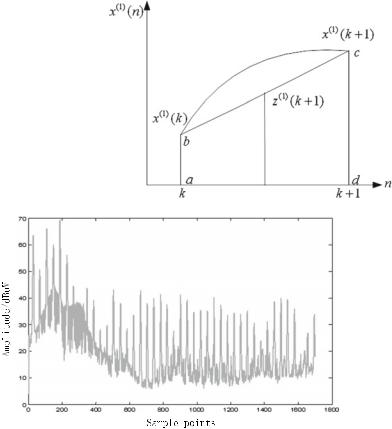
5.4 EMC Simulation Method |
233 |
Fig. 5.85 Accumulation generation and consecutive neighbor generation
Fig. 5.86 Original data sequence curve
We perform direct modeling and subsection modeling, respectively, of the original sequence and obtain the model curve as shown in Fig. 5.88. The errors in the direct modeling and the segmented modeling are calculated. The modeling error in Fig. 5.88a is 35.93%. In Fig. 5.88b, the modeling error becomes 28.75%. Therefore, when the consistency of the slope of one-accumulation generation curve is poor, as shown in Fig. 5.87a, we should use subsection modeling to achieve a better overall trend component fitting.
Based on the theoretical analysis and experimental validation, it can be seen that: Before modeling the overall trend component of the spectrum, we need to test whether the spectrum sequence needs to be segmented; if necessary, then we shall model the overall trend component in the segments. It is because that the segmented sequence shows a certain trend, and there is consistency among segments; we can use the GM (1, 1) model to build models for each of the (sm + 1) segments separately and obtain
(0) |
(0) |
(0) |
(0) |
}. Then, we sum up the |
the estimated value of each segment {xˆs1 |
, xˆs2 |
, · · · , xˆsm |
, xˆsm+1 |
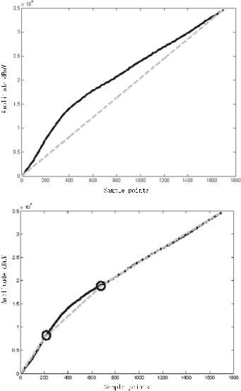
234 |
5 Critical Techniques of Quantitative System-Level EMC Design |
(a)
(b)
Fig. 5.87 Accumulation generation sequence
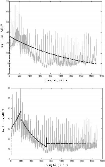
5.4 EMC Simulation Method |
235 |
(a)
(b)
Fig. 5.88 Modeling of the overall trend data sequence
236 5 Critical Techniques of Quantitative System-Level EMC Design
estimated value from the start to the end and obtain the estimation of the overall trend, i.e., X(0) (x(0)(1), x(0)(2), . . . , x(0)(n)), of the entire spectrum sequence that
X |
(x |
(1), x |
(2), . . . x(n)). |
needs to be analyzed, i.e., ˆ |
ˆ |
ˆ |
ˆ |
2. Harmonic frequency characteristics extraction from the spectrum
After extracting the overall trend component, the residual component can be considered as the emission component that has the main contribution in the spectrum. The analysis of these components is performed from both the frequency and the amplitude perspectives. Here, we will focus on the extraction of the frequency characteristics of harmonic interference components. On the one hand, the frequency of harmonic components can be extracted to determine the fundamental frequency to initially locate the interference source. On the other hand, the amplitude at the frequency point can be extracted based on the frequency information, which serves as the basis of the amplitude characteristics of the interference source.
The spectral data containing harmonics includes not only a fundamental wave component of a certain frequency but also a harmonic component of the fundamental frequency multiplication; therefore, the harmonic wave component is periodic. For such a data sequence, a gray system model and a periodic extension model need to be used at the same time. That is, the overall trend component in the spectrum is first modeled, and the modeling residual (the difference between the original test sequence and the GM (1, 1) model sequence) is modeled periodically.
The spectral residual sequence is obtained by removing the overall trend components in the test spectrum. It can be written as
x1 (k) |
|
x(0)(k) |
x(k) |
(5.220) |
|
|
− ˆ |
|
Based on the analysis of the physical meaning of the spectrum, before the residual series is modeled, the negative items in the series are set to zero to obtain a modified residual sequence x (k), which satisfies
x |
(k) |
|
x1 (k), x1 (k) ≥ 0 |
(5.221) |
|
|
|
0, |
x1 (k) < 0 |
|
|
Then, we can find the periodic extension model of the residual series x (k).
3. Harmonic amplitude characteristics extraction from spectrum
In the study of EMC, we can often derive the characteristics of the waveform that produce interference from the envelope characteristics of electromagnetic emission test data [65]. Therefore, this book adopts the Fourier envelope theory to analyze various types of radiation waveforms to obtain some simple rules.
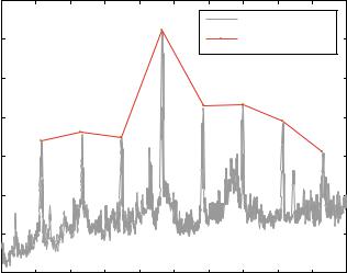
5.4 EMC Simulation Method |
237 |
90 |
|
|
|
|
|
|
|
|
|
|
|
|
|
|
|
|
|
Test Serial |
|
|
|
80 |
|
|
|
|
|
|
Amplitude of the |
|
||
|
|
|
|
|
|
Harmonic Component |
|
|||
|
|
|
|
|
|
|
|
|||
70 |
|
|
|
|
|
|
|
|
|
|
60 |
|
|
|
|
|
|
|
|
|
|
50 |
|
|
|
|
|
|
|
|
|
|
40 |
|
|
|
|
|
|
|
|
|
|
30 |
|
|
|
|
|
|
|
|
|
|
20 |
|
|
|
|
|
|
|
|
|
|
0 |
100 |
200 |
300 |
400 |
500 |
600 |
700 |
800 |
900 |
1000 |
Fig. 5.89 Harmonic component amplitude modification extraction
(1) Extraction of harmonic amplitude points
According to the previous analysis, the harmonic frequencies are obtained, and the corresponding frequencies are selected for amplitude extraction of the harmonic points. In this situation, the frequency during the measurement is obtained by discrete sampling, so the measured signal peak and the actual peak value may not be exactly the same in frequency, which can also cause deviations at the fundamental frequency. If this deviation is not taken into consideration, the deviation will increase with the increase of the multiple when calculating the fundamental frequency multiplication, which may result in incorrect results. For this reason, it is necessary to calculate the possible range of frequency instead of a simple frequency point. In practice, we can take the left and right ten frequency points of the selected signal frequency as the possible range of the signal frequency and select the signal peak in this range as the envelope of the harmonic components, as shown in Fig. 5.89.
(2) Modification of the radiation emission amplitude
It is almost impossible to restore the exact radiation field intensity generated by the original signal directly from the emission spectrum. Therefore, some simple formulas are used to describe the characteristics of the radiation field, and a certain modification is made to the test data to obtain the approximated characteristics of the emission source [66]. These simplifications include: keeping only the value of the field in the most suitable direction; aligning the receiving antenna with the direction of maximum polarization; assuming a uniform current distribution in the cable, it is acceptable to use an average equivalent current rather than the maximum; and ignoring the dielectric and impedance loss of the wire. In view of the above simplification, only
238 |
5 Critical Techniques of Quantitative System-Level EMC Design |
Fig. 5.90 Trapezoidal wave and its spectral envelope.
a Trapezoidal waves. b Spectrum envelope
the change in the slope of the envelope is used when analyzing the amplitude envelope of the harmonics. That is, only certain quantized characteristics of the waveform can be obtained, but the accurate amplitude values of the radiation source cannot be obtained. Practical applications show that the simplified formula can solve most practical problems.
(3) Quantitative characteristics of the harmonic spectrum amplitude
The corresponding amplitude for the extracted harmonic frequency points is obtained. The x-axis is then converted to a logarithmic coordinate, and the harmonic envelope is plotted. Then, we shall find the turning points on the envelope, from which the waveform characteristics of the corresponding source of harmonic components can be calculated.
Now, we consider the waveform shown in Fig. 5.90a. Its spectral envelope is shown in Fig. 5.90b. From the beginning to F1 1/π d, the envelope of the spectrum is constant, then decreases with a slope of −20 dB/dec until F2 1/π τr , and then falls again with a slope of −40 dB/dec.
The amplitude peak A (W, A, etc.), the pulse width d, the signal period T , and the rising time tr (the time corresponding to a signal amplitude change from 10 to 90%, and if the falling and rising times are different, the shorter one is selected as tr ) can be read from Fig. 5.90b. Therefore, once the envelope of the spectrum is obtained, some characteristics of the original waveform can be determined based on the slope turning points. The width of the pulse waveform can be obtained from the first slope turning point, and the rising time of the waveform can be calculated from the second
5.4 EMC Simulation Method |
239 |
turning point. If we can get all the exact values of the spectrum envelope, which is very difficult, we could also calculate the amplitude of the waveform.
4. Correspondence between the interference elements and the actual equipment
To connect the extracted interference elements with a certain device/circuit in the equipment to understand the constituent elements of the spectrum, it is necessary to correlate the characteristics of the interference elements. The corresponding of the characteristics is started with the frequency characteristics, and frequency match is directly compared. If there are no matching devices, the amplitude characteristics are then considered, as shown in Fig. 5.91. This way, the spectral characteristics obtained from the test can be completely matched with the characteristics of the device/circuit in the equipment.
5. Examples and verification of electromagnetic emission element identification
(1) Examples of conduction emission
This section analyzes three examples from different data analysis perspectives: The importance of modifying the residuals is explained through the light source system conduction analysis; the frequency of the harmonic components in the frequency spectrum is analyzed through the switching mode power supply (SMPS) conduction emission; through testing equipment with unknown internal composition, its frequency and amplitude are analyzed using the methods presented in this section. The measured data in this section was all obtained from testing.
(1)Conduction analysis of the light source system. In Fig. 5.92, the solid line shows the conduction emission (CE) measurement result of the positive line of a light source system’s power module. The dashed line is the overall trend component extracted using the method proposed in this book. The dashed line in Fig. 5.93 is a gray-periodic model obtained by directly modeling the residual sequence with an extracted periodic interval of 59.
The residual sequence is modified as shown in Eq. (5.221). Only harmonic components that contribute positively to the frequency spectrum are considered. Then, the sequence of the modified residual sequence is modeled as shown in the dashed line in Fig. 5.94. The extracted period of the model is 118. Since the frequency sampling interval set in the test is 5 kHz, the direct modeling harmonic frequency is 295 kHz and the error is 12.46%. Furthermore, the modified modeling harmonic frequency is 590 kHz and the error is reduced to 10.85%. If we want to further reduce the error of the model sequence, we can model the residual with negative values, but the results of the analysis do not contribute much to the understanding of the characteristics of the key components in the spectrum. Therefore, considering the result and efficiency, we do not perform more accurate spectrum modeling.
The switching frequency of the power module of the actual light source system is 590 kHz. It is obvious that the result after the above modification of the residual
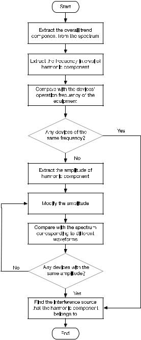
240 |
5 Critical Techniques of Quantitative System-Level EMC Design |
Fig. 5.91 Flowchart of the correspondence between the interference components and equipment
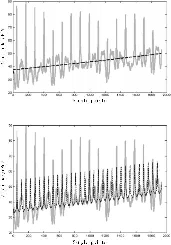
5.4 EMC Simulation Method |
241 |
Fig. 5.92 Light source system test spectrum sequence and overall trend modeling sequence
Fig. 5.93 Direct modeling of the spectral residuals of light source systems
better satisfies the accuracy requirement. It is also found that the cause of harmonics emission of the switch section is the insufficiency of the power supply filter. (2) Conduction emission analysis of SMPS. Figure 5.95 shows the frequency-domain conduction emission (CE102) measurement result of the SMPS’ positive line. The 250 kHz to 8.5 MHz part of the spectrum is modeled and analyzed, the x-axis frequency display is labeled with serial numbers, and then the spectrum analysis is performed.
First, we use the trapezoidal envelope of the spectrum to perform spectrum segmentation. The trapezoidal envelope shown in Fig. 5.96 in the dashed line is cal-

242 |
5 Critical Techniques of Quantitative System-Level EMC Design |
Fig. 5.94 Periodic modeling of residuals after modification
Amplitude/dbuV
Frequency / Hz
Fig. 5.95 SMPS power conduction emission (CE102) test result
culated using Eq. (5.219). The spectrum segments calculated from the difference sequence are listed in Table 5.17.
Table 5.17 shows that the two calculated frequency spectrum segmentation points are No. 200 and No. 700. Therefore, the spectrum shown in Fig. 5.96 will be modeled in three segments divided by these two segment points.
The gray GM (1, 1) model is used to model the overall trend component of the spectrum as shown by the dashed line in Fig. 5.97a. Then, we shall use the grayperiodic modeling method to extract the frequency of the harmonics and the obtained sequence interval is 40. The model is shown in Fig. 5.97b. Multiplying the sequence interval with the test interval of 4875 Hz, we can get a harmonic interval of 195 kHz.
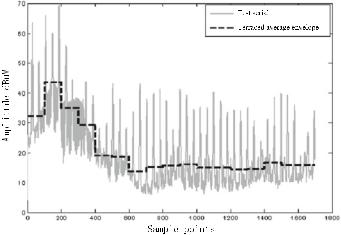
5.4 EMC Simulation Method |
243 |
Fig. 5.96 Test data sequence and the trapezoidal envelope
Table 5.17 Segmentations of the conduction spectrum of the power supply
Serial number of spectrum (*100) |
1 |
2 |
3 |
4 |
5 |
6 |
7 |
8 |
|
|
|
|
|
|
|
|
|
Trapezoidal envelope difference sequence |
1 |
0 |
0 |
0 |
0 |
0 |
1 |
1 |
|
|
|
|
|
|
|
|
|
Whether a segmentation point |
No |
Yes |
No |
No |
No |
No |
Yes |
No |
|
|
|
|
|
|
|
|
|
Serial number of spectrum (*100) |
9 |
10 |
11 |
12 |
13 |
14 |
15 |
16 |
|
|
|
|
|
|
|
|
|
Trapezoidal envelope difference sequence |
1 |
0 |
1 |
0 |
1 |
1 |
0 |
1 |
|
|
|
|
|
|
|
|
|
Whether a segmentation point |
No |
No |
No |
No |
No |
No |
No |
No |
|
|
|
|
|
|
|
|
|
Since the on–off frequency of the transistor of the SMPS under test is 195 kHz, it can be inferred that the excessive portion in the frequency spectrum is mainly caused by the frequent on–off of the transistor. Therefore, we can add a filtering device to the power supply end in the circuit including the transistor or add the power factor correction circuit to change the emission of harmonics.
(3)Conduction emission analysis of a rotary motor. The comparison of the conduction emission spectrum of a rotary motor and the emission limit is shown in Fig. 5.98. Spectral analysis is performed by extracting the spectrum from 10 k to 250 kHz that are severely over standard. The extracted frequency spectrum is shown in Fig. 5.99, where the dashed line is the trapezoidal curve obtained by dividing it into segments and averaging the segments.
The same calculation method as in the previous example is used to obtain the difference sequence represented by 0/1, as listed in Table 5.18.
According to the calculation procedure, only one segmentation point is selected which is also the first point of the sequence. Therefore, this spectrum does not need to be segmented. We can build its gray GM (1, 1) model as shown in Fig. 5.100.
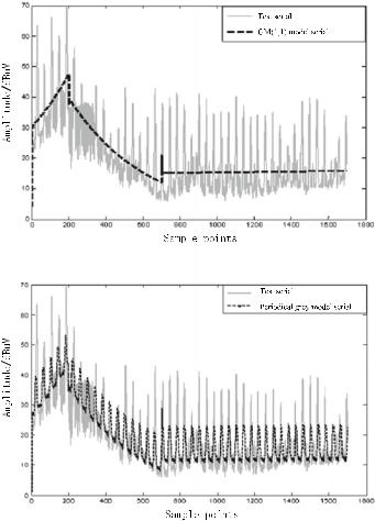
244 |
5 Critical Techniques of Quantitative System-Level EMC Design |
(a)
(b)
Fig. 5.97 Test data series and the overall trend components and the gray-periodic model sequence. a Test data series and the overall trend components. b Test data sequence and the gray-periodic model sequence
Table 5.18 Spectrum segmentations of the rotary motor
Serial number of spectrum (>100) |
1 |
2 |
3 |
4 |
5 |
6 |
7 |
8 |
9 |
|
|
|
|
|
|
|
|
|
|
Trapezoidal envelope difference |
1 |
1 |
1 |
1 |
1 |
0 |
1 |
0 |
0 |
sequence |
|
|
|
|
|
|
|
|
|
|
|
|
|
|
|
|
|
|
|
Whether a segmentation point |
Yes |
No |
No |
No |
No |
No |
No |
No |
No |
|
|
|
|
|
|
|
|
|
|
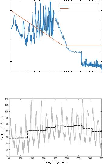
5.4 EMC Simulation Method |
245 |
|
110 |
|
|
|
|
|
|
PWM output, motor works |
|
|
100 |
|
Limit of CE102 |
|
|
|
|
|
|
|
90 |
|
|
|
dBuV |
80 |
|
|
|
/ |
|
|
|
|
|
|
|
|
|
Amplitude |
70 |
|
|
|
|
|
|
|
|
|
60 |
|
|
|
|
50 |
|
|
|
|
40 |
|
|
|
|
104 |
105 |
106 |
107 |
Frequency / Hz
Fig. 5.98 Comparison of output waveforms and the emission limit when the rotary motors with PWM are switched on
Fig. 5.99 Emission spectrum and its trapezoidal envelope of the rotary motor
Then, we build a periodic model of the residual sequence and add it to the gray GM (1, 1) sequence to get
x |
(0)(k) |
|
81.5775e0.00011(k−1) + f |
44 |
(k) |
(5.222) |
ˆ |
|
|
|
|
It can be seen from (5.222) that the period parameter is 44. Then, we multiply it with the spectrum test interval 300 Hz and get the fundamental frequency of the
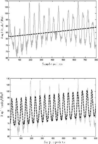
246 |
5 Critical Techniques of Quantitative System-Level EMC Design |
Fig. 5.100 Rotary motor test sequence and its overall trend component
Fig. 5.101 Test sequence and gray-periodic model sequence
harmonics as 13.2 kHz. The established model and original sequence are shown in Fig. 5.101.
The amplitude of the harmonic component is extracted. Since the data is obtained from the conduction test, no amplitude modification is required. The envelope of its harmonic component is drawn directly with logarithmic coordinates as shown in Fig. 5.102. Then, we can remove the outliers in the harmonics, trace the envelope of the harmonics using the thick line in Fig. 5.102, and detect the slope turning point of the tenfold octave in the envelope using Fourier envelope analysis.
The harmonic frequency is 13.2 kHz, and the conduction emission test starts at 10 kHz. Since the complete information of the waveform cannot be obtained,
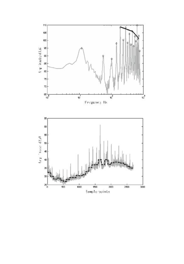
5.4 EMC Simulation Method |
247 |
Fig. 5.102 Harmonic envelope of the test sequence
Fig. 5.103 Test data and its trapezoidal envelope
only the second turning point frequency of 146.5 kHz can be detected, of which the corresponding waveform indicates that the pulse rising time is 2.2 μs. The rotating frequency of the rotary motor is 13.2 kHz, and the triggering time of the PWM wave that controls its rotation is extremely short, which is the same as the analysis result in this section. Therefore, we can conclude that the interference emissions in the spectrum are generated by the PWM signal. The overshoot of the conduction emissions can be improved by setting the PWM control chip. If we cannot change
248 |
5 Critical Techniques of Quantitative System-Level EMC Design |
Fig. 5.104 Test data and the overall trend components
the time to control its rotation, we can try better shielding the chip or filtering the output signal.
(2) Radiation emission examples
The electromagnetic interference generated inside the electronic equipment can radiate to the space through PCB, the internal interconnection wires within the equipment, and various interface cables connecting the equipment to the outside.
The examples analyze the emission spectrum of an electronic equipment containing one harmonic component and multiple harmonic components. The measured data was all obtained from the one-meter radiation emission test.
(1)Analysis of radiation emission of a piece of navigation equipment. The radiation emission spectrum of a piece of navigation equipment is shown in Fig. 5.103. The dashed line is the trapezoidal curve obtained by averaging the segments.
The envelope difference sequence is calculated as listed in Table 5.19.
Equation (5.219) is used to calculate the three turning points with 0/1. However, because the identifier of the second point is the same as the first point, it can be omitted. Thus, there are only two segmentation points remaining, of which one is the 600th point of the sequence, and the other is the 2200th point. The sequence is divided into three parts by the two points.
The GM (1, 1) model is established separately for these three parts, and then the segments are connected. Finally, the overall trend component of the spectrum sequence is obtained as shown in Fig. 5.104.
Then, combining the periodic model with the gray system model, we obtain a gray-periodic combination model. The parameter in the model is calculated to be
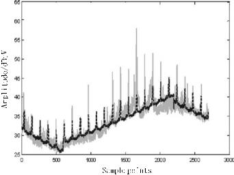
250 |
5 Critical Techniques of Quantitative System-Level EMC Design |
Fig. 5.105 Test sequence and the gray-periodic model sequence
x |
(0)(k) |
|
32.1701e−0.00034(k1 −1) |
|
ˆ |
|
|
|
|
|
|
+ 28.5493e0.00023(k2 −1) + 39.1213e−0.00023(k3 −1) |
|
|
|
|
+ f117(k) |
(5.223) |
|
The curve of the model sequence is shown in Fig. 5.105. It can be seen from the figure that the frequency of the harmonics obtained from the modeling agrees well with the actual measured curve. From (5.223), we can see that the periodic sequence interval is 117. Multiplying it with the test interval 47 kHz, we can get the fundamental frequency of the harmonic components as 5.5 MHz.
According to the obtained fundamental frequency information, we can get the amplitudes of the various harmonics. Then, we can use the “modification method of the radiation emission amplitude” in the section “harmonic amplitude characteristics extraction from spectrum” (case 3) to modify the amplitude. The spectrum and the values of the harmonics after modification are shown in Fig. 5.106a. Then, we draw the envelope and display it in logarithmic coordinates, as shown in Fig. 5.106b.
The fundamental frequency obtained from the modeling is 5.5 MHz. The radiation emission test starts from 3 MHz. Since the complete information of the waveform cannot be obtained, the information of the first turning point is lost. Only the second turning point of the envelope can be detected, and its corresponding frequency is 115.5666667 MHz. Based on the frequency value, we can calculate the rising time of the pulse waveform of the source and get a result of 2.75 ns. From the fundamental frequency information, the period of the waveform can be calculated as 181 ns. Assuming that the duty cycle of the waveform is 50%, it can be seen that the rising time of the pulse is too short, which leads to harmonic interference of the funda-
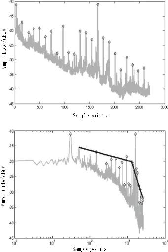
5.4 EMC Simulation Method |
251 |
(a)
(b)
Fig. 5.106 Harmonics and harmonic envelope curves of the test sequence. a Harmonics of the test sequence after modification and b harmonic envelope curves after modification
mental frequency in an extremely wide frequency band. During the troubleshooting procedure of EMC, we can suppress the harmonics of the output waveform of the crystal clock or increase the rising time. For the later production of this product, it is necessary to select a crystal with better performance during the design phase and perform better chip-level filtering.
(2)Spectrum analysis of multi-harmonic equipment. In some tests, the spectrum data may contain harmonics generated by a plurality of different fundamental
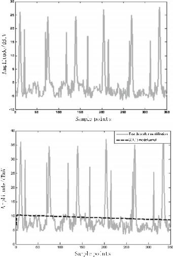
252 |
5 Critical Techniques of Quantitative System-Level EMC Design |
(a)
(b)
Fig. 5.107 GM (1, 1) model of the original test spectrum sequence (modified test sequence). a Original test spectrum sequence and b test sequence and the GM (1, 1) model
frequency components. For the analysis of this spectrum, a “multiple harmonic frequency extraction” method is used to extract the harmonic components of the spectrum.
First, we observe the test spectrum sequence which is shown in Fig. 5.107a. From the figure, we can see that the sequence is positive and negative staggered. Since the condition of gray modeling is that the sequence is nonnegative, and the effect of amplitude can be temporarily ignored when extracting the frequency characteristics, the minimum value in the spectrum sequence is detected as −6.3836. Therefore, the
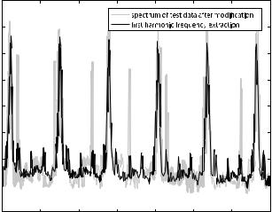
5.4 EMC Simulation Method |
253 |
|
40 |
|
|
|
|
|
|
|
|
35 |
|
|
|
|
|
|
|
|
30 |
|
|
|
|
|
|
|
/ dBuV |
25 |
|
|
|
|
|
|
|
|
|
|
|
|
|
|
|
|
Amplitude |
20 |
|
|
|
|
|
|
|
15 |
|
|
|
|
|
|
|
|
|
|
|
|
|
|
|
|
|
|
10 |
|
|
|
|
|
|
|
|
5 |
|
|
|
|
|
|
|
|
0 |
50 |
100 |
150 |
200 |
250 |
300 |
350 |
|
0 |
Sample points
Fig. 5.108 Test spectrum sequence and the first harmonic extraction after modification
values of the entire sequence are added by 10 to ensure that all values are nonnegative, as shown by the solid line in Fig. 5.107b. Then, the overall trend component of the modified sequence is modeled, and the fitting function of the GM (1, 1) model is
x |
(0)(k) |
|
(1 |
− |
ea )(x(0) |
(1) |
|
b |
)e−a(k−1) |
|
|
|
|
||||||||
ˆ |
|
|
|
|
− a |
(5.224) |
||||
|
|
|
10.2879e−0.0005(k−1) |
|||||||
|
|
|
|
|
|
|
|
|
|
|
The dominant period is calculated using the method of variance analysis in combination with the maximum deviation square sum between each group and the mean value, and the simulation sequence shown in Fig. 5.108 is obtained. This sequence contains a harmonic with an interval of 64. The amplitude of the harmonic component in the sequence containing a single harmonic of the model is set to be a random value within the range of the total trend component, and the range is calculated using Eq. (5.224) to be (6.8175, 10.2826). Therefore, we set the harmonic of cycle 64 to follow the uniform distribution of U (5, 11).
The resulting new model sequence is shown in Fig. 5.109.
The second harmonic of the new spectrum sequence is extracted to obtain a period that satisfies the conditions of variance analysis. The serial number is 48. The result of the second harmonic extraction is shown as the dashed line in Fig. 5.109.
The superposition of the two harmonics is compared with the original test spectrum sequence, as shown in Fig. 5.110. No other dominant period is found after detection of the residual sequence. At this point, the harmonic extraction modeling process ends.
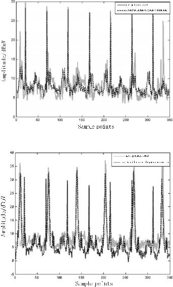
254 |
5 Critical Techniques of Quantitative System-Level EMC Design |
Fig. 5.109 New spectrum sequence and the second harmonic extraction
Fig. 5.110 Comparison of the original test spectrum sequences with multiple harmonic extractions