

108 |
5 Critical Techniques of Quantitative System-Level EMC Design |
5.3 EMC Modeling Methodology
5.3.1 Methodology of System-Level Modeling
The information system is a complex system with a wide frequency band, complex signal forms, and various coupling relationships. System-level EMC modeling needs to be performed from the perspective of system modeling.
1. Concept of system
Ideally, a system usually refers to a study object, an associated object, or a closed-loop system that includes a predictor. A system is independent from its “environment”; i.e., although a system is affected by the environment, it has its own characteristics and may even have an impact on the environment. The impact of the environment on the system is regarded as an input of the system. The relationship between the input and output of the system is determined by the characteristics of the system itself as shown in Fig. 5.4. The inputs and outputs of the system that change over time are called input and output variables. If the system has only one input and one output variable, it is called a single-input and single-output (SISO) system. Similarly, if the system has multiple independent input and output variables, the system is called a multi-input and multi-output (MIMO) system.
In practical applications, a system may be affected by various factors from the outside. Therefore, the three elements of the system (entities, attributes, and activities) and the environment need to be determined before we study the system any further. The system is determined only if the entities, attributes, activities, and environment are clearly defined.
2. System classification
According to different criteria, the system can be classified into linear systems and nonlinear systems; deterministic systems and stochastic systems; time-invariant systems and time-varying systems; constraint systems and unconstrained systems; continuous-state systems and discrete-state systems; continuous-time systems and discrete-time systems; time-driven systems and event-driven systems; lumped parameter systems and distributed parameter systems; systems with computer networks (intelligent systems) and systems without computer networks, etc.
Most of the systems involved in the field of EMC are characterized by nonlinearity, uncertainty, time-varying, constrained, and with distributed parameters, and they are mostly continuous-time systems. It can be predicted that the intelligent systems will become mainstream with computers taking the role of process control. Thus, complex intelligent networks will also be involved by EMC in the future.
Fig. 5.4 Mutual influence between system and environment
5.3 EMC Modeling Methodology |
109 |
3. Definition of system model
A model is a logical representation of a system in physics, mathematics, or other modes. It provides knowledge about the system in a certain form (such as words, symbols, diagrams, objects, mathematical formulas). The system model, on the one hand, reflects the main characteristics of the actual system, and on the other hand, is a higher-level abstraction that can be applied to similar problems.
Therefore, a good system model should have three characteristics: It is the abstraction or imitation of the real system; it is composed of the main factors that reflect the nature or characteristics of the system; it is the concentration of the relationship between the main factors.
In most cases, the system model is not the system itself, but a description of the essential attributes of a certain aspect of the system. The system is complex, and its attributes are also multifaceted. Therefore, the model can be classified into static model and dynamic model according to the time dependencies; it can be classified into “black box” model and “white box” model according to whether the internal characteristics of the system are described; it can be classified into deterministic model, random model, continuous model, discrete model according to the form of variables; it can be classified into algebraic equation model, differential (difference, iterative) equation model, statistical model, and logical model according to the relationship between variables.
In engineering systems, we often encounter systems with numerous state variables, complex feedback structures, and nonlinear characteristics of inputs and outputs. These systems are called complex systems. When these characteristics are directly used as the main features of the system, they are correspondingly referred to as high-order systems, multi-loop systems, nonlinear systems, and network systems. If the number of subsystems in a complex system is large with many types and complex relationship among each other, the system is called a complex giant system. Although such systems have objectively defined characteristics, the differences in subsystems will result in variations.
4. System modeling principles
Firstly, we will introduce the concept of homomorphism and isomorphism in system modeling. Assume system A has an input signal A(t), and system S has an input signal B(t), where t ≥ 0. Isomorphic systems are systems that have the same reaction to external excitation. For two isomorphic systems, same input will produce same output. If the input signal set and output status set of system B only correspond to a few representative inputs and outputs of system A, then system B is said to be a homomorphic system of system A. An isomorphic system must be homomorphic, but the reverse is not necessarily true.
Modeling means building the isomorphism and homomorphism of the prototype. The interaction between the entities of the system will cause its attribute to change. Entities and attributes of the system may change at different times. The change is usually described as states. At any moment, all information about entities, attributes, and activities in the system is called the state of the system at that moment. The variables representing the system state are called state variables.
110 |
5 Critical Techniques of Quantitative System-Level EMC Design |
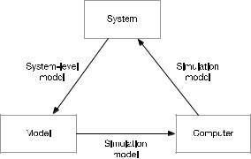
Fig. 5.5 Relationship of the three elements in system-level modeling and simulation
An ideal model for a prototype system should be a “good” homomorphic system. “Good” means that the model catches the important state that determines the system performance. Based on the analysis and research of the system, an ideal model shall be object-oriented and be built with deep understanding of the system’s working environment.
System modeling and simulation include three basic activities: system modeling (primary modeling), simulation modeling (secondary modeling), and simulation testing. The three activities are connected by the three elements of the computer simulation: system, model, and computer (including hardware and software). The relationship between the three elements of system modeling and simulation is shown in Fig. 5.5.
5.3.2 Methodology for Behavioral Modeling
The system-level EMC problem usually contains multiple crossover EMI and multiple modes of interference coupling associating with each other. All of the subsystems, equipment, or circuit modules contained in an electronic information system have physical circuit structures. However, for a system design engineer, it is difficult to build a full simulation model for the physical structure of an electronic system. The global simulation calculation of the underlying physical circuit in the system is the bottleneck in current system simulation [22].
The top-down system-level EMC quantitative design technique is to evaluate the EMC of the system by means of simulation tests, simulation calculations, etc., and to quantitatively allocate and optimize the design [14]. This top-level EMC predesign requires a simulation technique that is in a higher level than that of the transistors and devices. The predesign method can quickly put down the indicator requirements of each subsystem or circuit module from top to bottom. Behavioral modeling technology is undoubtedly an important method for system-level EMC analysis. The simplified mathematical model is used to describe the functional characteristics of
5.3 EMC Modeling Methodology |
111 |
each subsystem and circuit module, simplify the underlying physical structure of the circuit, increase the simulation speed, and reduce the computational cost.
As described in Sect. 4.3.7, EMC behavioral modeling is a modeling method that targets the external behavior of the system. Therefore, behavioral modeling needs to go through conceptual description, modeling, and verification.
To build a system-level EMC behavioral model, we usually use layered simulation methods to establish a suitable model and select an appropriate simulation tool. EMC models have two categories: One is for extracting parameters; the other is for solving field and energy distribution problems. The purpose of distinguishing these two is to choose the appropriate modeling tool.
A system-level EMC behavioral model generally includes the behavioral model of subsystems/equipment/components (including susceptive unit, interference sources), coupling channel models (including radiation and conduction), and equivalent models of environmental factors. Despite the tight coupling involved in multiple domains, EMC system modeling often involves the solving of nonlinear transmission equations.
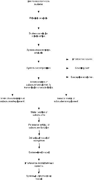
Figure 5.6 illustrates the EMC behavioral modeling method, which is an effective EMC modeling method.
5.3.2.1Concept Description of EMC Based on System Characteristics
Before establishing a system-level EMC behavioral model, the concept description of EMC based on system characteristics should be completed first. The main purpose of the concept description is to (1) establish the overall technical framework for the system-level EMC of the object according to its intended functions; (2) formulate the principle of collaborative control and determine the overall work content; (3) summarize the major concerns; and (4) sort out the key control indicators. Then, we can determine the workflow, make a timetable, establish a staff network, and finally establish a conceptual model of system-level EMC.
(1)Establish an overall technical framework: Position the system-level EMC of the objects to be designed. Through the positioning, all parties can understand the levels, time frame, participating institutions and personnel, funding requirements, risks, etc., of the system-level EMC of the object.
(2)Formulate the principle of collaborative control: Formulate collaboration strategies in terms of time, participating institutions and personnel, and funding. In the same time, determine the collaborative interaction protocols in terms of technology, interfaces, data, and resources.
(3)Determine the overall work package: In technical, testing, controlling, managing, and archiving level, sort out and specify the lifecycle work package in terms of design, development, evaluation, production, and application.
(4)Summarize major concerns: Summarize the major technical difficulties, important control objects, and major coordination issues.
112 |
|
|
5 Critical Techniques of Quantitative System-Level EMC Design |
|||||||||
|
|
|
|
|
|
|
|
|
|
|
|
|
|
|
|
|
|
|
|
|
|
|
|
|
|
|
|
|
|
|
|
|
|
|
|
|
|
|
|
|
|
|
|
|
|
|
|
|
|
|
|
|
|
|
|
|
|
|
|
|
|
|
|
|
|
|
|
|
|
|
|
|
|
|
|
|
|
|
|
|
|
|
|
|
|
|
|
|
|
|
|
|
|
|
|
|
|
|
|
|
|
|
|
|
|
|
|
|
|
|
|
|
|
|
|
|
|
|
|
|
|
|
|
|
|
|
|
|
|
|
|
|
|
|
|
|
|
|
|
|
|
|
|
|
|
|
|
|
|
|
|
|
|
|
|
|
|
|
|
|
|
|
|
|
|
|
|
|
|
|
|
|
|
|
|
|
|
|
|
|
|
|
|
|
|
|
|
|
|
|
|
|
|
|
|
|
|
|
|
|
|
|
|
|
|
|
|
|
|
|
|
|
|
|
|
|
|
|
|
|
|
|
|
|
|
|
|
|
|
|
|
|
|
|
|
|
|
|
|
|
|
|
|
|
|
|
|
|
|
|
|
|
|
|
|
|
|
|
|
|
|
|
|
|
|
|
|
|
|
|
|
|
|
|
|
|
|
|
|
|
|
|
|
|
|
|
|
|
|
|
|
|
|
|
|
|
|
|
|
|
|
|
|
|
|
|
|
|
|
|
|
|
|
|
|
|
|
|
|
|
|
|
|
|
|
|
|
|
|
|
|
|
|
|
|
|
|
|
|
|
|
|
|
|
|
|
|
|
|
|
|
|
|
|
|
|
|
|
|
|
|
|
|
|
|
|
|
|
|
|
|
|
|
|
|
|
|
|
|
|
|
|
|
|
|
|
|
|
|
|
|
|
|
|
|
|
|
|
|
|
|
|
|
|
|
|
|
|
|
|
|
|
|
|
|
|
|
|
|
|
|
|
|
|
|
|
|
|
|
|
|
|
|
|
|
|
|
|
|
|
|
|
|
|
|
|
|
|
|
|
|
|
|
|
|
|
|
|
|
|
|
|
|
|
|
|
|
|
|
|
|
|
|
|
|
|
|
|
|
|
|
|
|
|
|
|
|
|
|
|
|
|
|
|
|
|
|
|
|
|
|
|
|
|
|
|
|
|
|
|
|
|
|
|
|
|
|
|
|
Fig. 5.6 EMC behavioral modeling methodology
5.3 EMC Modeling Methodology |
113 |
(5)Sort out the key control indicators: According to the characteristics of the objects to be designed, sort out the effective technical indicators.
(6)Determine the complete workflow: Develop the EMC workflow chart and the corresponding logs.
(7)Making a timetable: Monitor the milestones through the entire developing process.
(8)Establishing a staff network: Establish the appropriate technical team and management team with clear responsibilities, work packages, and smooth information exchange.
The specific technical works involved in the concept description stage are: (1) Sort out the main radiation sources and susceptive equipment in the system, and annotate the attributes (transmitter, receiver, transceiver); (2) sort out the energy transmission relations from field, field–circuit, circuit to susceptive equipment, and build system interference relationships; (3) list the factors affecting EMC in the interference relationships; i.e., list the main EMC indicators of each equipment, for example, the overall planning of frequency resource between radiation equipment and susceptive equipment, electromagnetic environment, transmitter performance (transmission frequency, transmitting power, harmonic suppression, out-of-band suppression), receiver performance (receiving frequency, receiver susceptibility, adjacent channel suppression, out-of-band suppression), antenna layout performance (antenna patterns, polarization characteristics, antenna isolation), suppression capabilities, equipment and cable layout, interconnection characteristics (band coupling, shielding effectiveness, power usage, and grounding), and damage threshold. The output of the concept description based on the EMC of system characteristics is a conceptual model that can be used to analyze the key attributes of the system.
Assume a system with several pieces of transmitting equipment through antenna ports, other radiation equipment, receiving equipment coupled through antenna ports, and other susceptive equipment. Part of the radiation sources and susceptive equipment in a system are listed in Table 5.1, and the energy transfer relationships among the equipment are shown in Table 5.2. The main factors affecting the isolation between transmitting and receiving antennas are shown in Table 5.3.
When describing the concept of system EMC, it is important to sort out the spectral characteristics of the interference source. The EMI spectrum of the interference source can be categorized into the main interference spectrum and the out-of-band interference spectrum. It is generally believed that the radiation power of the interference source in the main interference spectrum accounts for most of its total transmission power.
The power spectral distribution of the interference source is
PN , f < fmin |
|
p( f ) PB , fmin < f < fmax |
(5.30) |
PT , f > fmax
114 |
5 Critical Techniques of Quantitative System-Level EMC Design |
||
Table 5.1 Part of the radiation source and susceptive equipment |
|
||
|
|
|
|
Indicator |
|
Equipment |
Operation state |
|
|
|
|
1 |
|
EMI transmitter |
Transmitter |
|
|
|
|
2 |
|
TCAN |
Transmitter/receiver |
|
|
|
|
3 |
|
Shortwave radio |
Transmitter/receiver |
|
|
|
|
4 |
|
Radio altimeter (RADALT) |
Transmitter/receiver |
|
|
|
|
5 |
|
Weather radar |
Transmitter/receiver |
|
|
|
|
6 |
|
Transponder |
Transmitter/receiver |
|
|
|
|
7 |
|
Autopilot system |
Transmitter/receiver |
|
|
|
|
8 |
|
Radio compass |
Receiver |
|
|
|
|
9 |
|
VOR receiver |
Receiver |
|
|
|
|
10 |
|
Microwave landing system |
Receiver |
|
|
|
|
11 |
|
Localizer receiver |
Receiver |
|
|
|
|
12 |
|
Flight data recorder |
Susceptive equipment |
|
|
|
|
13 |
|
Power supply parameter display |
Susceptive equipment |
|
|
|
|
14 |
|
Fuel gauge |
Susceptive equipment |
|
|
|
|
where PB is the power spectrum of the EMI emitted by the interference source in its main interference band; PN and PT are the power spectrum of the EMI emitted by the interference source outside its interference band; f min and f max are the lower band and upper band of the main interference spectrum, respectively.
The types of interference sources can be classified into broadband interference model, narrowband interference model (single-frequency interference model), harmonic interference model, and impulse interference model.
1. Broadband interference model
When the interference bandwidth is greater than the bandwidth of narrowband communication system, it belongs to the broadband interference. The spectrum of the broadband interference model is generally expressed as a function of spectral density, i.e.,
PN , PT ( f ),
p( f ) PB ( f ), PT ( f ), PN ,
f <
fT L fB L fB H
f <
fT L |
|
|
< f < fB L |
|
|
< f |
< fT H |
(5.31) |
< f |
< fT H |
|
fT H |
|
|
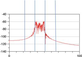
where PT (f ) is the power spectral density of the transition zone; f TL and f TH are the cutoff frequency of the lower sideband transition zone and the cutoff frequency of the upper sideband transition zone, respectively.
The output spectrum of the broadband interference model is shown in Fig. 5.7.
5.3 EMC Modeling Methodology |
|
|
115 |
||
Table 5.2 Energy transmission among part of the equipment |
|
|
|||
|
|
|
|
|
|
Indicator |
Transmitter |
Type of |
Specific |
Susceptive |
Coupling |
|
|
transmitting |
transmitting |
equipment |
position of |
|
|
node |
position |
|
susceptive |
|
|
|
|
|
equipment |
|
|
|
|
|
|
1 |
EMI |
Antenna type |
Antenna |
Shortwave |
Antenna |
|
transmitter |
|
|
radio |
|
|
|
Antenna |
Cable |
||
|
|
|
|
||
|
|
|
|
|
|
|
|
|
RF |
|
Antenna |
|
|
|
transmission |
|
|
|
|
|
line |
|
|
|
|
|
|
|
|
|
|
|
Power line |
|
Antenna |
|
|
|
|
|
|
|
|
Cable type |
Power line |
|
Cable |
|
|
|
|
|
|
|
|
Slot type |
Case |
|
Antenna |
|
|
|
|
|
|
|
|
|
Case |
|
Cable |
|
|
|
|
|
|
|
|
Grounding |
Power ground |
|
Power ground |
|
|
system |
|
|
|
|
|
Power ground |
|
Signal ground |
|
|
|
|
|
||
|
|
|
|
|
|
2 |
EMI |
Antenna type |
Antenna |
Radio |
Sensor |
|
transmitter |
|
|
altimeter |
|
|
|
Antenna |
Cable |
||
|
|
|
|
||
|
|
|
|
|
|
|
|
|
RF |
|
Sensor |
|
|
|
transmission |
|
|
|
|
|
line |
|
|
|
|
|
|
|
|
|
|
|
Power line |
|
Sensor |
|
|
|
|
|
|
|
|
Cable type |
Power line |
|
Cable |
|
|
|
|
|
|
|
|
|
RF |
|
Cable |
|
|
|
transmission |
|
|
|
|
|
line |
|
|
|
|
|
|
|
|
|
|
Slot type |
Case |
|
Cable |
|
|
|
|
|
|
|
|
|
Case |
|
Sensor |
|
|
|
|
|
|
3 |
EMI |
Antenna type |
Antenna |
Autopilot |
Cable |
|
transmitter |
|
|
system |
|
|
Cable type |
RF |
Cable |
||
|
|
|
|||
|
|
|
transmission |
|
|
|
|
|
line |
|
|
|
|
|
|
|
|
|
|
|
Power line |
|
Cable |
|
|
|
|
|
|
|
|
Slot type |
Case |
|
Cable |
|
|
|
|
|
|
|
|
Grounding |
Power ground |
|
Power ground |
|
|
system |
|
|
|
|
|
|
|
|
|
116 5 Critical Techniques of Quantitative System-Level EMC Design
Table 5.3 Influencing factors for isolation between receiver and transmitting antenna of carrier system
Indicator |
|
1 |
|
|
2 |
|
|
3 |
|
|
|
|
|
|
|
|
|
|
|
|
|
|
|
Transmitting antenna |
|
T1 |
T2 |
T3 |
|||||||
|
|
|
|
|
|
|
|
|
|
|
|
Receiving antenna |
|
R1 |
R2 |
R3 |
|||||||
|
|
|
|
|
|
|
|
|
|
|
|
Frequency |
Frequency (MHz) |
|
|
|
|
|
|
|
|
|
|
|
|
|
|
|
|
|
|
|
|
|
|
|
Transmit attributes |
|
|
|
|
|
|
|
|
|
|
|
|
|
|
|
|
|
|
|
|
|
|
|
Receive attributes |
|
|
|
|
|
|
|
|
|
|
|
|
|
|
|
|
|
|
|
|
|
|
Isolation by testing (dB) |
|
|
|
|
|
|
|
|
|
|
|
|
|
|
|
|
|
|
|
|
|
|
|
Parameters of transmitting |
Transmit peak power (dBm) |
|
|
|
|
|
|
|
|
|
|
antenna |
|
|
|
|
|
|
|
|
|
|
|
Gain of transmitting antenna |
|
|
|
|
|
|
|
|
|
|
|
|
|
|
|
|
|
|
|
|
|
|
|
|
(dB) |
|
|
|
|
|
|
|
|
|
|
|
|
|
|
|
|
|
|
|
|
|
|
|
Attenuation of transmitting |
|
|
|
|
|
|
|
|
|
|
|
band (dB) |
|
|
|
|
|
|
|
|
|
|
|
|
|
|
|
|
|
|
|
|
|
|
Parameters of receiving antenna |
Gain of receiving antenna (dB) |
|
|
|
|
|
|
|
|
|
|
|
|
|
|
|
|
|
|
|
|
|
|
|
Attenuation of receiving band |
|
|
|
|
|
|
|
|
|
|
|
(dB) |
|
|
|
|
|
|
|
|
|
|
|
|
|
|
|
|
|
|
|
|
|
|
|
Receiving sensitivity (dBm) |
|
|
|
|
|
|
|
|
|
|
|
|
|
|
|
|
|
|
|
|
|
|
Parameters of polarization |
Polarization |
|
|
|
|
|
|
|
|
|
|
|
|
|
|
|
|
|
|
|
|
|
|
|
Polarization mismatch (dB) |
|
|
|
|
|
|
|
|
|
|
|
|
|
|
|
|
|
|
|
|
|
|
Spatial isolation (Ld/dB) |
|
|
|
|
|
|
|
|
|
|
|
|
|
|
|
|
|
|
|
|
|
|
|
Antenna isolation |
|
|
|
|
|
|
|
|
|
|
|
|
|
|
|
|
|
|
|
|
|
|
|
Fig. 5.7 Output spectrum of broadband interference model
Wideband Interferance / dB
Pass band Main band Pass band
Frequency / MHz
5.3 EMC Modeling Methodology
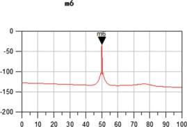
Fig. 5.8 Output spectrum of the narrowband interference model
Single Frequency Interferance / dB
117
Frequency = 50 MHz
Single Frequency Interferance = 33.369 dB
Frequency / MHz
2. Narrowband interference model
When the interference bandwidth is much smaller than the bandwidth of the communication system, it belongs to narrowband interference. In the analysis frequency range, frequency interference is similar to the single-frequency interference. The spectrum of the interference model is generally the frequency band energy function at a certain frequency resolution.
PN , |
f < fB |
|
p( f ) PB , |
f fB |
(5.32) |
PN , |
f > fB |
|
where f B is the current interference frequency and PB is the output power of the frequency point. The output spectrum of the narrowband interference model is shown in Fig. 5.8.
3. Harmonic interference model
Interference components that occur at certain frequency intervals are harmonic interference. In the behavioral modeling, we can represent the single-frequency interference component of the frequency cycle distribution as
PN , |
f |
|
fH · k |
|
p( f ) PB (k), |
f |
fH · k |
(5.33) |
|
PN , |
f |
|
fH · kB |
|
where f H is the fundamental frequency of the harmonic interference and PB(k) is the output power of the k-th harmonic frequency.
Figure 5.9 shows the output spectrum of the harmonic interference model.
4. Pulse interference model
Common pulse sources include nuclear pulses, lightning pulses, and static pulses. Electronic equipment also generates pulse currents when they are switched on/off and when their working conditions change. Due to its wide spectrum, flexibility, and
118
Fig. 5.9 Output spectrum of the harmonic interference model
5 Critical Techniques of Quantitative System-Level EMC Design
Frequency = 8 MHz |
Frequency = 8 MHz |
Harmonic Interferance = -47.157 |
Harmonic Interferance = -47.157 |
Harmonic Interferance / dB
Frequency / MHz
pertinence, pulse interference is usually high frequency and high energy that instantly exceeds the safety threshold of the electronic devices and equipment. Therefore, the pulse interference has a very strong ability to destroy electronic systems such as communications, radar, and computer networks. The electromagnetic pulse is random and abrupt, and it becomes a major research direction for electromagnetic protection.
The characteristics of the pulse interference are related to its form in time domain. Thus, to build a behavioral model of the pulse interference, we need to establish a time-domain model first and then re-analyze its time–frequency characteristics. In this book, the typical pulse interference models are the rectangular pulse model, exponential decay pulse model, and damped sinusoidal pulse model. The main parameters of the pulse model are start time, delay time, end time, and decay time (for attenuation-type pulses only).
For example, the rectangular pulse model has a time-domain representation function as
0, |
t < 0 |
|
V (t) V0, 0 < t < T |
(5.34) |
|
0, |
t > T |
|
where V 0 is the pulse amplitude and T is the pulse end time, respectively.
The typical output of time domain and frequency domain for the rectangular pulse model, exponential decay pulse model, and damped sinusoidal pulse model is showed in Fig. 5.10, Fig. 5.11, and Fig. 5.12, respectively.

5.3 EMC Modeling Methodology |
|
119 |
Rectangular Pulse / V |
Frequency Spectrum of |
Pulse / mV |
Time / ns |
|
Frequency / MHz |
Fig. 5.10 Time-domain and frequency-domain output of rectangular pulse model |
||
Exponential Decay Pulse / V |
Frequency Spectrum of |
Pulse / mV |
Time / ns |
|
Frequency / MHz |
Fig. 5.11 Time-domain and frequency-domain output of exponential decay pulse model |
||
Damped Sine Pulse / V |
Frequency Spectrum of |
Pulse / mV |
Time / ns |
|
Frequency / MHz |
Fig. 5.12 Time-domain and frequency-domain output of damped sinusoidal pulse model
5.3.2.2EMC Behavioral Modeling
A behavioral model is the quantification of a conceptual model. Formal modeling languages and various modeling tools can be used to build an executable abstract model. Behavioral modeling can be further divided into behavioral modeling based on equipment characteristics and behavioral modeling based on interference correlation matrix. Since the nonlinearity is an important cause of the complexity of EMC problems, we will specifically analyze the behavioral modeling methods for nonlinear systems at the end of this section.
1. Behavioral modeling based on equipment characteristics
EMC behavioral modeling based on equipment characteristics is to directly integrate the equipment behavioral models of each system or subsystem together to form a

120 |
5 Critical Techniques of Quantitative System-Level EMC Design |
(a)
(b)
Transmitter
(c)
Signal
Source
Amp Filter
Matched Mixer signal
source
Scan frequency analysis
|
|
Antenna isolation |
|
|
|
|
Receiver |
|
|
|
Isolation equivalent |
|
|
|
|
|
|
|
|
network |
|
|
|
|
|
|
|
|
|
|
|
|
Capacitor |
Capacitor |
|
|
|
|
|
|
|
|
|
|
|
|
|
|
Resistor |
Resistor |
|
|
Bias |
Signal |
|
|
|
|
|
|
Capacitor |
|
|
|
|
|
|
Resistor |
voltage |
||
|
|
|
|
|
|
|||
Source |
|
S parameter simulation |
Capacitor |
|
Capacitor |
|
|
|
Amp |
|
|
|
|
||||
Filter |
Resistor |
|
|
Inductor |
|
|
|
|
|
|
|
|
|
|
|
|
|
Mixer |
|
Capacitor |
Power divider |
|
Filter |
Inductor |
|
|
|
|
|
|
Power |
|
|||
|
|
|
|
|
|
Filter |
Capacitor |
|
|
|
Matched |
|
Filter |
|
divider |
||
|
|
|
|
|
|
|
|
|
Harmonic analysis |
load |
|
Two-port network |
|
|
Filter |
|
|
|
|
|
|
|
|
Matched |
|
|
Filter |
load |
|
|
Filter |
|
|
|
|
Fig. 5.13 EMC behavioral model of an airborne transceiver system based on equipment characteristics. a Geometry model of airborne transmitters and receivers; b isolation between transmitting and receiving antennas; and c EMC behavioral model of an airborne transceiver system
system-level or subsystem-level behavioral model. In the behavioral model based on equipment characteristics, we only consider the one-way energy flow between equipment, without considering the complex multiple coupling relationships between equipment. Although the model built this way might suffer from some errors, the modeling process is simple and clear. Therefore, we still consider the model to be effective for the first rough analysis.
We will use Fig. 5.13 as an example to illustrate the EMC behavioral modeling based on the equipment characteristics: Fig. 5.13a is the geometry model of an airborne transceiver system. The coupling relationship between the transmitting and the receiving antennas can be determined during concept description. Only the transmitting system needs to be considered in the EMC behavioral modeling based on equipment characteristics.
The behavioral model of the receiving system and the antenna coupling model (frequency characteristics of the antenna isolation) between the transmitting and the receiving antenna is shown in Fig. 5.13b. When the relationship between the antenna
5.3 EMC Modeling Methodology |
121 |
isolation and the frequency is substituted by the equivalent magnitude–frequency network, we obtain the behavioral model as shown in Fig. 5.13c. Thus, we can see that the behavioral model shown in Fig. 5.13c is a direct integration of the transmitter-side behavioral model, the receiver-side behavioral model, and the isolation model. The complex coupling relationship between the transmitting and the receiving antennas is not taken into account into the behavioral modeling.
To establish the EMC behavioral model for equipment as shown in Fig. 5.13c (such as the transmitting system and the receiving system behavioral model), we can adopt the idea of node analysis: Based on the principle of circuit configuration of EMI source and electromagnetic susceptive object, the equivalent circuit model can be simulated to obtain the external behavioral response of the equivalent circuit model. Then, we can build the EMC behavioral model of the equipment based on the functional indicator correction.
We will use the behavioral model of shortwave radio as an example to explain the method of behavioral modeling of the equipment’s EMC in the transmitter or the receiver as illustrated in Fig. 5.13c.
Shortwave radios generally have high transmission power and are often the main source of interference to other equipment.
Based on the analysis of the EMI characteristics among various pieces of equipment in the system, when modeling the behavior of a shortwave radio station, the focus is to simulate its interference characteristics of externally generated radiation.
(1) Requirement analysis for shortwave radio station
As a transmitting equipment, the fundamental frequency of a shortwave radio station will affect other equipment operating in the same frequency in the system. The harmonics and broadband noise generated by the radio frequency power amplifier will interfere with other highly susceptive receiving equipment.
Since the load of the shortwave radio power amplifier’s last transistor cannot reach the optimum at each frequency in the wide band, in order to obtain the same large output power, the transistor may be working in saturation region or cutoff region when the load is not in a frequency band of optimal state. This will cause large nonlinear distortion, and a series of harmonics and broadband noise.
If harmonics exist in a shortwave radio station, the efficiency of energy transmission and energy utilization will be reduced, the equipment will be overheated, noise will be generated, the insulation of the radio stations will be deteriorated, and the life of the equipment will be shortened. Harmonics can even result in the radio station failure or burnout. What’s more, harmonics may cause partial parallel resonance or series resonance of the system; thus, the harmonic content increases and the capacitor and other equipment might be burned. Therefore, when modeling the harmonic characteristics of a shortwave radio station, it is necessary to consider both the simulation of the normal operation of the radio station itself and the simulation of the external interference. CE106 project requirements in GJB 151 can be referred to modeling.
The wideband noise generated by the shortwave radio stations is an important cause of the interference from the radio stations toward the external sensitive receiv-
122 |
5 Critical Techniques of Quantitative System-Level EMC Design |
ing equipment. Since the broadband noise exists in a frequency band between the main frequency and the harmonics and it is close to the fundamental and harmonic waves, it is difficult to use filters or other technical means to separate or eliminate the noise. The broadband noise produced by shortwave radios is mainly due to nonlinearity, which mainly are the harmonics and intermodulation signal produced by the transmitting equipment.
(2) Modeling process
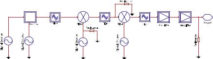
The superheterodyne structure is used in the shortwave radio transmission equipment, and an equivalent model can be established on the circuit simulation software platform according to the circuit principle of the shortwave radio station: Firstly, build an emission model to analyze its external radiation characteristics; secondly, build models for the typical sub-modules including AM module, mixer module, and nonlinear transmission module.
(1)Establish a transmission model. The basic parameters needed to establish the transmission model are frequency range, frequency interval, work type, output power, harmonic attenuation, IF selectivity, harmonic rejection ratio, etc. The transmission model scheme is as follows. Firstly, the radio frequency carrier signal is modulated by the modulation signal and the impedance of modulator is set. Secondly, the signal is up-converted by the first local oscillator and the first IF signal is obtained after the filter. Then, after up-converted by the second local oscillator, the output frequency point is moved to the transmission carrier frequency. Finally, after amplified by a small-signal amplifier and a power amplifier, the output fundamental wave signal in frequency domain can be obtained which satisfies the power demand. The shortwave radio transmission model is shown in Fig. 5.14.
(2)Establish models for typical sub-modules. The main modules in the transmission model are AM module, mixer module, and nonlinear transmitter module. The model of the nonlinear transmitter module is the most important, since it determines the core functional indicators of the shortwave radio RF port.
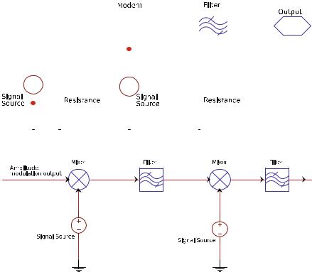
AM module. Since the original signal is in low frequency, it is generally not suitable for direct transmission. Therefore, it is necessary to perform signal modulation. The most common analog modulation methods are amplitude
Fig. 5.14 Transmission model of a shortwave radio station
5.3 EMC Modeling Methodology |
123 |
modulation and angle modulation using a sine wave as carrier. The shortwave radio behavioral model exploits amplitude modulation methods such as amplitude modulation (AM), double-sideband modulation (DSB), vestigial sideband modulation (VSB), and single-sideband modulation (SSB).
Amplitude modulation: The amplitude of the sinusoidal carrier changes linearly with the modulation signal, i.e.,
Sm (t) F[sm (t)] A[M(ω − ωc) + M(ω + ωc)]/2 |
(5.35) |
Double-sideband modulation: If the input baseband signal has no DC component and h(t) is an ideal band-pass filter, then the resulting output signal is a double-sideband modulated signal without a carrier component, which can also be called a double-sideband modulation signal. If the input baseband signal has a DC component and it is also assumed to be an ideal band-pass filter, then the resulting output signal is a double-sideband signal with a carrier component.
Single-sideband modulation: The double-sideband modulated signal contains two sidebands, the upper and lower sidebands. Since these two sidebands contain the same information, from the perspective of information transmission, it is enough to transmit only one sideband. Single-sideband modulation is a modulation method that produces only one sideband.
Residual sideband modulation: It is a linear modulation between the double sideband and single sideband. It not only overcomes the shortcomings of bandwidth occupied by the double-sideband modulated signal, but also solves the problem of implementing single-sideband signal. This method partially suppresses one sideband instead of completely suppressing; thus, a small portion of the sideband remains.
When establishing the AM sub-module model, we need to consider the RF carrier signal frequency and the modulation signal frequency. The AM sub-module behavioral model is shown in Fig. 5.15.
Mixer module. The basic functions of the mixer are up-conversion and down-conversion. Up-conversion mixes the IF signal with the RF oscillation signal into the new RF signal and transmits it through the antenna; the down-converter is used to mix the RF signal received by the antenna with the local carrier signal and filter it into IF signal. Then, the IF signal is sent to the IF processing module. In the conversion process, the modulation type (regardless of amplitude modulation, frequency modulation, or phase modulation) and the modulation parameters (such as modulation frequency, number of modulations, etc.) do not change, and only the signal carrier frequency is changed. According to the principle of the mixer, the mixer
behavioral model can be built as shown in Fig. 5.16.
Nonlinear emission module. Equipment that causes nonlinearity in shortwave radios usually has mixers, filters, amplifiers, and so on. We will focus on the behavioral model of the power amplifier module.
124 |
|
|
|
|
|
|
|
|
|
|
|
|
|
|
|
5 Critical Techniques of Quantitative System-Level EMC Design |
||||||||||||||||||||
|
|
|
|
|
|
|
|
|
|
|
|
|
|
|
|
|
|
|
|
|
|
|
|
|
|
|
|
|
|
|
|
|
|
|
|
|
|
|
|
|
|
|
|
|
|
|
|
|
|
|
|
|
|
|
|
|
|
|
|
|
|
|
|
|
|
|
|
|
|
|
|
|
|
|
|
|
|
|
|
|
|
|
|
|
|
|
|
|
|
|
|
|
|
|
|
|
|
|
|
|
|
|
|
|
|
|
|
|
|
|
|
|
|
|
|
|
|
|
|
|
|
|
|
|
|
|
|
|
|
|
|
|
|
|
|
|
|
|
|
|
|
|
|
|
|
|
|
|
|
|
|
|
|
|
|
|
|
|
|
|
|
|
|
|
|
|
|
|
|
|
|
|
|
|
|
|
|
|
|
|
|
|
|
|
|
|
|
|
|
|
|
|
|
|
|
|
|
|
|
|
|
|
|
|
|
|
|
|
|
|
|
|
|
|
|
|
|
|
|
|
|
|
|
|
|
|
|
|
|
|
|
|
|
|
|
|
|
|
|
|
|
|
|
|
|
|
|
|
|
|
|
|
|
|
|
|
|
|
|
|
|
|
|
|
|
|
|
|
|
|
|
|
|
|
|
|
|
|
|
|
|
|
|
|
|
|
|
|
|
|
|
|
|
|
|
|
|
|
|
|
|
|
|
|
|
|
|
|
|
|
|
|
|
|
|
|
|
|
|
|
|
|
|
|
|
|
|
|
|
|
|
|
|
|
|
|
|
|
|
|
|
|
|
|
|
|
|
|
|
|
|
|
|
|
|
|
|
|
|
|
|
|
|
|
|
|
|
|
|
|
|
|
|
|
|
|
|
|
|
|
|
|
|
|
|
|
|
|
|
|
|
|
|
|
|
|
|
|
|
|
|
|
|
|
|
|
|
|
|
|
|
|
|
|
|
|
|
|
|
|
|
|
|
|
|
|
|
|
|
|
|
|
|
|
|
|
|
|
|
|
|
|
|
Fig. 5.15 Behavioral model of AM sub-module
Fig. 5.16 Behavioral model of the mixer
RF power amplifier is an important part of nonlinear transmission equipment. In the transmitter’s prestage circuit, the power of the RF signal generated by the modulation circuit is very small, and it needs to go through a series of amplification, such as the buffer level, the intermediate amplifier level, and the final power amplifier level. After sufficient RF power is obtained, it can be sent to the antenna. Therefore, RF power amplifiers must be used to obtain sufficient RF output power.
In the transmission system, the output power of the RF power amplifier mainly refers to the output power of the final-stage power amplifier. In order to achieve high-power output, the prefinal stage must already have sufficient power levels for excitation. Its main technical indicators are output power and efficiency. At the same time, the harmonic components in the output should be as small as possible to avoid generating interference toward other channels.
According to the different current conduction angles, the RF power amplifier can be categorized into three classes, which are Class A, Class B, and Class C. In addition, there are Class D and Class E amplifiers in which the electronic devices operate in the on–off state.
5.3 EMC Modeling Methodology |
125 |
Filter’s Output |
|
|
Output |
Amplifier |
Amplifier |
|
Resistance |
Fig. 5.17 |
Behavioral model of the nonlinear transmission part |
|
|
||
Input |
Probe |
AGC |
Filter |
Probe |
Output |
|
|
Amplifier |
|
|
|
|
|
|
|
|
|
Fig. 5.18 |
Behavioral model of final-stage power amplifier |
|
|
|
|
In terms of the characteristics of the amplifier, the key parameters are gain and gain flatness, operating frequency and bandwidth, output power, DC input power, input/output reflection coefficient, and noise coefficient. In addition, other parameters such as intermodulation distortion (IMD), harmonics, feedback, and thermal effects are often considered. All of these parameters can seriously affect the performance of the amplifier.
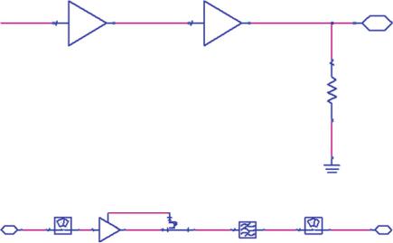
The modeling scheme is designed as follows: The signal input to the final power amplifier is firstly passed through a small-signal amplifier, and the transmitted small signal is amplified to the required magnitude; after that, the signal is adjusted through the final power amplifier, which is the main component of the nonlinear emission model to meet the requirement of shortwave radio transmission power. The behavioral model of the nonlinear emission part is shown in Fig. 5.17. The behavioral model of the final-stage power amplifier is shown in Fig. 5.18.
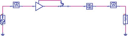
When the first-stage amplifier in the model shown in Fig. 5.17 fails to meet the requirement of the actual transmitting power, the final-stage power amplifier can be designed using automatic gain control and automatic power control technology. The automatic gain control can automatically control the amplitude of the gain by changing the input and output compression ratio. It maintains the amplitude of the output signal or keeps the signal changing within a small range when the amplitude of the input signal varies greatly. Therefore, the system can operate properly with very low input signal, and the receiver will not be saturated or jamming due to the input signal being too large. The behavioral model of automatic gain control amplifier is shown in Fig. 5.19.
126
Matched Signal Source |
Probe |
|
5 Critical Techniques of Quantitative System-Level EMC Design
|
AGC |
|
Probe |
Amplifier |
|
Filter |
LoadMatched |
|
|
Fig. 5.19 Behavioral model of automatic gain control amplifier
Based on the behavioral models presented above, we can simulate and predict the spurious emissions (including harmonic emission and broadband noise) generated by a shortwave radio.
Before modeling subsystem or systems with multiple equipment, we need to consider the interference coupling problems among equipment; in other words, we need to establish a model of interference coupling transmission path. In behavioral modeling based on equipment characteristics, the model of interference coupling transmission path only includes one-way energy flow between equipment, regardless of the multiple and complex coupling relationships between equipment.
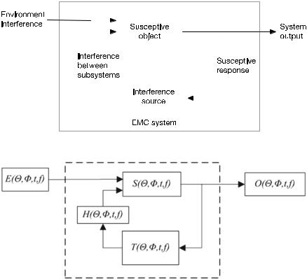
Now, we will discuss an example of the model of interference coupling transmission path which is shown in Fig. 5.20. The system is composed of a susceptive object and an interference source (the susceptive object and the interference source are subsystems which are composed of several lower-level subsystems. We can get more detailed coupling relationships by identifying the input and output variables of these lower-level subsystems). Each of the input and output variables is marked with an arrow indicating its direction of interference. The EMI generated by the interference source acts on the susceptive object and is an input variable for the susceptive object. In addition to the internal sources of interference, external environmental interference also affects the entire system and acts on the susceptive object, which can be considered as another input variable for the susceptive object. At the same time, the response of a susceptive object may have a counter-effect on the interference source. This effect is not necessarily interference, but it may determine whether the interference source or even the whole aircraft can continue to work normally or not.
When building the model of interference coupling transmission path, special attention must be paid to the direction of the transmission path between subsystems and the change in energy in the transmission direction. The EMC behavioral model describes the dynamic process of interference coupling by a path transfer function. The transfer function can be determined by frequency response test or numerical calculation.
Figure 5.21 shows the interference coupling model based on the transfer function, where T ( , , t, f ) represents the interference source model; H ( , , t, f ) represents the interference coupling path model; S( , , t, f ) represents the suscep-
5.3 EMC Modeling Methodology |
127 |
||||||||
|
|
|
|
|
|
|
|
|
|
|
|
|
|
|
|
|
|
|
|
|
|
|
|
|
|
|
|
|
|
|
|
|
|
|
|
|
|
|
|
|
|
|
|
|
|
|
|
|
|
|
|
|
|
|
|
|
|
|
|
|
|
|
|
|
|
|
|
|
|
|
|
|
|
|
|
|
|
|
|
Fig. 5.20 Model of interference coupling transmission path of an electronic system
Fig. 5.21 Interference coupling model based on the transfer function
tive object model; E( , , t, f ) represents the environmental EMI source model; O( , , t, f ) represents the interference output model.
Figure 5.21 The interference coupling model based on the transfer function. where t and f represent the change of system characteristics with time and frequency; and represent other factors that affect the system characteristics.
EMC can be predicted based on the interference source model, interference coupling path model, susceptive object model, environmental EMI source model, etc. For the sake of simplicity, and are not considered for now. Then, the interference model T (t, f ) represents any interfering equipment with radiation or conduction emission characteristics in the system. The susceptive model S(t, f ) represents any equipment with radiationor conduction-susceptive characteristics within the system. The coupling function H(t, f ) represents the radiation coupling coefficient and the conduction coupling coefficient, which are mainly the coupling of the radiation field to the cable, the coupling between the cables, and the common power coupling. The signal coupled with the susceptive equipment is
128 |
5 Critical Techniques of Quantitative System-Level EMC Design |
|
|
R(t, f ) T (t, f ) × H (t, f ) |
(5.36) |
If I(t, f ) represents the interfering state discriminant function (safety margin function) of the susceptive equipment, then I(t, f ) can be expressed as
I (t, f ) R(t, f ) − S(t, f ) |
(5.37) |
The performance of the susceptive equipment can be evaluated by the value of
I (t, f ):
a.If I (t, f ) > 0, it means that the susceptive equipment will be interfered, and the value of I (t, f ) indicates the strength of the interference at the same time.
b.If I (t, f ) 0, it means that the susceptive equipment is in a critical state of interference. The equipment may suffer from interference, and the safety margin is 0.
c.If −6 < I (t, f ) < 0, it means that the susceptive equipment has not been interfered but is vulnerable to interference.
d.If I (t, f ) < −6, it means that the susceptive equipment will not be interfered and can work safely and stably.
2. Behavioral modeling based on interference correlation matrix
(1) System-Level Energy Coupling Model
The system’s energy coupling model is used to study the interference signal energy coupled with the susceptive equipment.
Assume the number of radiation source ports in the system is M2, in which there is M1 transmitting equipment whose front end is connected to the antenna. Since each transmitting equipment may have multiple radiation source ports (including the emission ports formed by the radiation of the antenna), usually M2 ≥ M1. The radiation sources that emit radiation emission through the transmitting antenna ports are denoted as E1, E2, . . . , EM1 ,and the other radiation source ports are denoted as EM1 +1, . . . , EM2 . Similarly, the number of the equivalent susceptive ports to be analyzed in the system (including fuses for pyrotechnics) is N2, and the number of receiving equipment whose front ends are connected to the antenna is N1. Since the energy transmitted by the emission source may be coupled with each receiving equipment through multiple ports (including the energy radiated by the radiation source through the receiving antenna port), it can be derived that N2 ≥ N1. The susceptive ports formed by the coupling of the receiving antenna ports are labeled as R1, R2, . . . , RN1 ,and other susceptive ports are labeled as RN1 + 1, . . . , RN2 .
In the environment of a system, the total power [23, 24] from the radiation source port coupled with the susceptive port in the frequency range fa fb is
PR ji |
fb ηi ( f )β j ( f ) |
d f |
(5.38) |
|
fa |
Ii j ( f ) |
|||

5.3 EMC Modeling Methodology |
129 |
where ηi ( f ) is the output power spectral density of the radiation source port i; β j is the response function of the susceptive port to different modulation signals; Ii j is the isolation between the radiation source port i and the susceptive port j.
The total power received by the susceptive port j from the radiation source is
( f ) ( f )
fb |
M2 |
fb η ( f )β |
j |
( f ) |
|
|
|||
|
|
i |
|
|
|
d f |
(5.39) |
||
PR j fa |
|
|
|
|
|||||
fa |
Ii j ( f ) |
||||||||
|
i 1 |
|
|
|
|
|
|
|
|
The electromagnetic radiation received by fuel, ordnance, and personnel is an important topic in system-level EMC analysis and prediction. Therefore, it is necessary to study the energy coupling model at the fuel inlet, ordnance, and work chamber of the aircraft.
The total power from the radiation source port to the fuel susceptive point in the frequency range fa fb is
PO ji |
fb ηi ( f )ξ j ( f, T ) |
d f |
(5.40) |
|
fa |
Ti j ( f ) |
|||
where the values of fa and fb may refer to the corresponding national military standard [25, 26]; Ti j ( f ) is the power transfer function of the radiation port i to the fuel inlet j; ξ j ( f, T ) is the electromagnetic power absorption rate of the fuel and gas mixture, which is determined by the frequency, time, temperature, density of the fuel and gas mixture, the flow speed of air, and other factors.
The total power received by the electromagnetic radiation source at the fuel susceptive point j is
fb |
M2 |
fb η ( f )ξ |
j |
( f, T ) |
|
|
||
|
|
i |
|
|
d f |
(5.41) |
||
PO j fa |
|
|
|
|||||
fa |
Ti j ( f ) |
|||||||
|
i 1 |
|
|
|
|
|
|
|
The total power from the radiation source port to the operator’s workstation in the frequency range fa fb is
fb |
|
fb |
ηi ( f ) |
(5.42) |
|
|
|||||
PW ji fa |
fa |
Ti j ( f, t) |
d f |
||
where the values fa , fb may refer to the corresponding military standards [27]; Ti j ( f ) is the power transfer function from the transmitting equipment i to the operator workstation j. It is a function of frequency and time.
The total electromagnetic radiation power at the operator’s workstation j is
fb |
M2 |
fb |
ηi ( f ) |
|
|
|
|
(5.43) |
|||
PW j fa |
fa |
|
d f |
||
Ti j ( f, t) |
|||||
|
i 1 |
|
|
|
|
130 |
5 Critical Techniques of Quantitative System-Level EMC Design |
(2) System-Level Interference Correlation Matrix
The interference correlation matrix describes the energy coupling relationship among the equipment in the system. In this section, we will establish the isolation matrix, antenna isolation matrix, transmitting power matrix of the transmitters, attenuation matrix of the transmitters at the frequency point to be analyzed, transmitting feeder loss matrix of the transmitters, sensitivity matrix of the receivers, and reception suppression matrix of the receivers at the analysis frequency point, receiving feeder loss matrix of the receivers, signal-to-noise ratio matrix required when the receivers operate normally, EMC safety margin matrix required by the receiving equipment, transmitting conversion matrix, receiving conversion matrix, safety threshold matrix of antenna isolations, interference power matrix of the receiver antenna ports.
Assuming the one-to-one correspondence between the radiation source port and the susceptive port, the relationship matrix between the radiation source port and the susceptive port of the entire system is
(E1, R1) · · · (E1, RN1 ) · · · (E1, RN2 )
. |
. |
. |
. |
. |
. |
. |
. |
. |
(EM1 , R1) · · · (EM1 , RN1 ) · · · (EM1 , RN2 ) , i [1, M2], j [1, N2] (5.44)
. |
. |
. |
. |
. |
. |
. |
. |
. |
(EM2 , R1) · · · (EM2 , RN1 ) · · · (EM2 , RN2 )
where (Ei , R j ) represents the energy transfer relationship between the radiation source port Ei and the susceptive port R j .
The energy transfer function between the radiation source port and the susceptive port describes the interference relationship and the strength of interference between the two ports.
The isolation between the radiation source port and the susceptive port is a one- to-one correspondence, and it exhibits as a power transfer function. Therefore, considering the safety of susceptive equipment, the interference matrix of the susceptive equipment is constructed with isolation Ii j ( f ) as elements. The antenna isolation matrix is
I11( f )
.
.
.
I (Ii j ( f )) Ii1( f )
.
.
.
IM2 1( f )
· · · I1 j ( f )
.
.
.
· · · Ii j ( f )
.
.
.
· · · IM2 j ( f )
· · · I1N2 ( f )
.
.
.
· · · Ii N2 ( f )
.
.
.
· · · IM2 N2 ( f )
5.3 EMC Modeling Methodology |
|
131 |
|
I (E1, R1) · · · I (E1, RN1 ) · · · I (E1, RN2 ) |
|
||
. |
. |
. |
|
. |
. |
. |
|
. |
. |
. |
|
I (EM1 , R1) · · · I (EM1 , RN1 ) · · · I (EM1 , RN2 ) , i [1, M2], |
j [1, N2] |
||
. |
. |
. |
|
. |
. |
. |
|
. |
. |
. |
|
I (EM2 , R1) · · · I (EM2 , RN1 ) · · · I (EM2 , RN2 ) |
(5.45) |
||
|
|
|
|
We can rewrite it in the form of dB |
|
||
|
|
I(dB) 10l g I |
(5.46) |
The sub-matrix A in the matrix I is the antenna isolation matrix, which represents the degree of isolation between the transmitter and the receiver when energy is transmitted through the antenna ports. We can take ideal values for the isolation of the equipment used for both transmitting and receiving, i.e.,
I (E1, R1)
.
.
.
A I (Ei , R1)
.
.
.
I (EM1 , R1)
· · · I (E1, R j )
.
.
.
· · · I (Ei , R j )
.
.
.
· · · I (EM1 , R j )
· · · I (E1, RN1 )
.
.
.
· · · I (Ei , RN1 )
.
.
.
· · · I (EM1 , RN1 )
, i [1, M1], j [1, N1]
(5.47)
where the isolation I (Ei , R j ) between the transmitting antenna i and the receiving antenna j is determined by factors such as the radiation characteristics of the transmitting and the receiving antennas, the mounting position in the system, the electrical size between the transmitting and the receiving antennas, the shielding condition, and the polarization matching between the transmitting and the receiving antennas. The antenna isolation matrix is an important topic in antenna layout optimization.
We can rewrite (5.47) in the form of dB
A(dB) 10lg A |
(5.48) |
The transmitting power matrix of the transmitters is |
|
Pt1 |
|
. |
|
. |
|
. |
|
Pt Pti (d Bm), i [1, M1] |
(5.49) |
. |
|
. |
|
. |
|
Pt M1
132 5 Critical Techniques of Quantitative System-Level EMC Design
where Pti is the transmitting power of the i-th transmitting equipment.
The emission attenuation matrix of the transmitters at the analysis frequency is
Lt B1( f )
.
.
.
LtB Lt Bi ( f ) (d Bc), i [1, M1] |
(5.50) |
.
.
.
Lt B M1 ( f )
where Lt Bi ( f ) is the amount of emission attenuation of the i-th transmitting equipment at the analysis frequency point and it is a function of the frequency. We can assume Lt Bi ( f ) 0dB within the emission bandwidth. Out of operation bandwidth, Lt Bi ( f ) represents the out-of-band attenuation and harmonic attenuation, and the data can be estimated using theoretical methods or obtained from tests.
The transmitting feeder loss matrix of the transmitters is
Lt f 1( f )
.
.
.
Ltf Lt f i ( f ) (dB), i [1, M1] |
(5.51) |
.
.
.
Lt f M1 ( f )
where Lt f i ( f ) is the RF transmission loss of the i-th transmitter. It indicates the feeder loss between the transmitter output port and the input port of the transmitting antenna. Similarly, it is a function of frequency.
Transmission line loss consists of transmission line length loss, waveguide discontinuity loss, rotating joint loss, connection failure loss, and transceiving switching loss (transceiving switching loss exists if the same antenna is used for both transmitting and receiving). At the same time, transmission line loss can only be relatively determined after system installation. The value should be 0.5–3.5 dB under most conditions.
The sensitivity matrix of the receivers is
Psmin [ Ps1 · · · Ps j · · · Ps N1 ](dBm), j [1, N1] |
(5.52) |
where Ps j is the design sensitivity of the j-th receiving equipment.
The reception suppression matrix of the receivers at the analysis frequency is
LrB [ Lr B1( f ) · · · Lr B j ( f ) · · · Lr B N1 ( f ) ](dBc), j [1, N1] |
(5.53) |
where Lr B j ( f ) is the reception suppression of the j-th receiving equipment at the analyzing frequency and it is a function of the frequency. We can assume Lr B j ( f ) 0dB
5.3 EMC Modeling Methodology |
133 |
within the receiver’s operating bandwidth. Outside the operating bandwidth, Lr B j ( f ) represents the out-of-band suppression of the receiver, harmonic suppression, etc. As with the data for Lt Bi ( f ), the data for Lr B j ( f ) can also be estimated using the methods provided in Chap. 3, but the test data is the best to use here.
The receiving feeder loss matrix of the receivers is
Lrf [ Lr f 1( f ) · · · Lr f j ( f ) · · · Lr f N1 ( f ) ](dB), j [1, N1] |
(5.54) |
where Lr f j ( f ) is RF transmission loss of the j-th receiving equipment. It is the transmission loss of the transmission line between the transmitting antenna output port and the receiver input port. It is also a function of frequency.
The signal-to-noise ratio (SNR) matrix required when the receivers operate normally is
|
|
|
S |
|
|
|||||||
|
|
|
|
( |
S |
)1 · · · ( |
S |
) j · · · ( |
S |
)N1 (dB), |
j [1, N1] |
(5.55) |
|
|
|
N |
N |
N |
N |
||||||
where ( |
S |
) j is the SNR of the j-th receiving equipment. |
|
|||||||||
N |
|
|||||||||||
The EMC safety margin required by the receiving equipment is |
|
|||||||||||
|
|
|
Sm [ Sm1 · · · Sm j · · · Sm N1 ](dB), |
j [1, N1] |
(5.56) |
|||||||
where Sm j is the EMC safety margin required for the j-th receiving equipment to operate normally, and the value may be 6 dB or 16.5 dB.
The transmitting conversion matrix is a 1 × M1 matrix. It can be expressed as
T E [1, 1, · · · , 1] |
(5.57) |
The receiving conversion matrix is an N1 × 1 matrix. It can be expressed as
1
1
TR . (5.58)
.
.
1
Considering the one-to-one correspondence between the transmitting equipment and the receiving equipment, if the entire system needs to fully meet the EMC requirements, it must be ensured that the receiver will not be interfered or desensitized. The safety threshold matrix of antenna isolations is then defined as
Alimit(dB) ( Alim it )
( Pt − Lt B − Lt f ) T E − ( P smi n + Lr B + Lr f − Sm) T R
(5.59)
134 5 Critical Techniques of Quantitative System-Level EMC Design
where is the Kronecker product; P t is the transmitting power matrix of the transmitters [Eq. (5.49)]; Lt B is the emission attenuation matrix of the transmitters at the analysis frequency [Eq. (5.50)]; Lt f is the transmitting feeder loss matrix of the transmitters [Eq. (5.51)]; P smi n is the sensitivity matrix of the receivers [Eq. (5.52)]; Lr B is the reception suppression matrix of the receivers at the analysis frequency (Eq. 5.53); Lr f is the receiving feeder loss matrix of the receivers (Eq. 5.54); Sm is the EMC safety margin matrix required by the receiving equipment (Eq. 5.56); T E is the transmitting conversion matrix (Eq. 5.57); T R is the receiving conversion matrix (Eq. 5.58).
It is worth mentioning that Eq. (5.95) is the optimal threshold for EMC design. Satisfying this equation means that the signals emitted by other transmitting equipment in the system will not interfere with the receiver through the antenna ports. Of course, the interference phenomenon does not necessarily occur if (5.95) is not satisfied. For a receiving equipment, as long as (5.60) and (5.61) are satisfied at the same time, the receiver can work normally. But it might be desensitized, and the
corresponding tactical and technical indicators might also decline. |
|
|||||
|
Ps j |
|
≥ ( |
S |
|
|
|
|
|
)m j |
(5.60) |
||
|
Jj + N j |
N |
||||
|
Ps j |
≥ Psmin |
(5.61) |
|||
where Ps j is the signal power received by the receiver j; Jj is the external interference power received by the receiver j; N j is the internal noise power of the receiver j. For a particular receiver, the value of N j is relatively stable.
In fact, for each receiver, any spectral component will be affected by any transmitting equipment in the system, but the degree of influence will be different. Considering that the receiver is affected by all transmitting equipment (through antennaradiated power), the interference power matrix coupled with the receiver antenna port is
J A [ J1 · · · Jj · · · JN1 ]
10l g T E 10 |
(Pt −LtB −Ltf ) TE−(LrB +Lrf ) TR −A(dB) |
(i [1, M1], j [1, N1]) (dB m) |
|
10 |
|||
|
|
||
|
|
(5.62) |
where 10A 10[I (Ei ,R j )] [10I (Ei ,R j )] (a matrix power of a constant). Considering that the power radiated from all sources is coupled with the susceptive
equipment, besides the antenna port, the coupled port can also be a slot, apertures, cable, or other interference channels. Based on different coupling approaches, the interference power coupled with other susceptive ports can be calculated using the same method to obtain JN1 +1, · · · , JN2 . The safety threshold of corresponding port isolation is I .
The energy transfer relationship between the radiation source port and the susceptive port described in Eq. (5.44) can also be described in the following way.
5.3 EMC Modeling Methodology |
135 |
It is assumed that the number of equipment in the system is M, and each equipment is regarded as a radiation source E( f ) with a constant radiation state or a periodic change. For example, the i-th equipment is expressed as Ei ( f )(i 1, 2, . . . , M), which indicates that the number of ports that can interfere with the outside is M. When the system is relatively large, several pieces self-contained equipment can be combined into subsystems to simplify the decomposition of the system. However, when the equipment is in an unstable state, the equipment should be further decomposed until it reaches a stable state.
Similarly, assuming that there are N receiving ports in the system and each port is denoted by R( f ), we define the j-th receiving port as R j ( j 1, 2, . . . , N )and the coupling function between the j-th receiving port and the i-th interference port as Hi, j ( f ). Then, the component of the total interference that may be received by the j-th receiving port is
R j ( f ) E1 |
( f ) · · · Ei ( f ) · · · EM ( f ) 1 M × |
|
× |
M |
|
H1, j ( f )
.
.
.
Hi, j ( f )
.
.
.
HM, j ( f ) M×1
Ei ( f )Hi j ( f ) |
(5.63) |
i 1 |
|
We can derive that the total interference received by all receiving ports within the entire electronic information system is
R1( f ) |
|
|
H1,1( f ) |
|
|
. |
|
. . . |
|
|
. |
|
|
. |
|
R j ( f ) |
E1 |
( f ) · · · Ei ( f ) · · · EM ( f ) 1 M × |
Hi,1( f ) |
. . . |
|
× |
. |
|
|
. |
|
RN ( f ) |
|
|
. |
|
|
HM,1( f ) |
|
|
|
|
M
· · · |
H1, j ( f ) |
. |
|
|
. |
|
. |
Hi, j ( f )
|
. |
|
. |
· · · |
. |
|
HM, j ( f )
· · · |
H1,N ( f ) |
. |
|
|
. |
|
. |
Hi,N ( f )
|
. |
|
. |
· · · |
. |
|
HM,N ( f ) M×N
Ei ( f )Hi,1( f )
|
i 1 . |
|
|
. |
|
|
. |
|
|
M |
(5.64) |
Ei ( f )Hi, j ( f ) |
i 1
.
.
.
M
Ei ( f )Hi,N ( f )
i 1
where the M × N matrix is called the interference correlation matrix I. It represents the coupling among different ports in the system and can be expressed as
136 |
5 Critical Techniques of Quantitative System-Level EMC Design |
|||||
|
H1,1( f ) |
· · · |
H1, j ( f ) |
· · · |
H1,N ( f ) |
|
|
. |
. |
. |
|
||
|
. |
|
. |
|
. |
|
I |
. |
|
. |
|
. |
|
Hi,1( f ) |
|
Hi, j ( f ) |
|
Hi,N ( f ) |
(5.65) |
|
|
. |
|
. |
|
. |
|
|
. |
|
. |
|
. |
|
|
. |
· · · |
. |
· · · |
. |
|
|
HM,1( f ) |
HM, j ( f ) |
HM,N ( f ) |
|
||
The coupling function between the i-th interference port and the j-th receiving port is Hi,j( f ).
When there are multiple coupling relationships (such as multi-path effects in communication) among subsystems and equipment in the system, there is no longer a one-to-one correspondence between the interference ports and the receiving ports; in other words, there is correlation among different interfering ports or receiving ports. Under this circumstance, we need to take the coupling factors brought by the correlation into consideration. In the following paraphrase, we will analyze the coupling relationship between multiple interference sources and a single receiving port in the system.
Assuming an electronic information system, the number of transmitting equipment (ports) is M and the number of susceptive equipment (ports) is N, and if there is correlation between the interference sources, the EMI coupled with the j-th susceptive object’s input port can be written as
|
M |
|
|
R j ( f ) Hji ( f ) × Ei ( f ) j 1 · · · N |
(5.66) |
||
|
i 1 |
|
|
|
|
|
|
If the susceptive limit of the j-th receiving port is Sj ( f ), its interference state function can be written as
I j ( f ) R j ( f ) − Sj ( f )
|
|
|
M |
|
|
|
|
Hji ( f ) × Ei ( f ) − Sj ( f ) |
(5.67) |
||
|
|
|
i 1 |
|
|
where |
M |
means that the transmission value is not directly arithmetically added, |
|||
i 1 |
|||||
|
|
|
|
|
|
and the interference calculation at the port cannot be simply calculated using the sum of the system functions. We also need to take into account the correlation function between the interference variables and the correlation function between the coupling transfer functions.
In EMC analysis, it is usual to find that multiple interference sources are uncorrelated, multiple transmission paths are uncorrelated, or the interference source functions and transmission path functions are uncorrelated. Since the output functions of the independent systems are uncorrelated, R j ( f ) can be expressed by the energy of the interference signal that the port couples with as
5.3 EMC Modeling Methodology |
|
|
137 |
M |
Hji ( f ) × Ei ( f ) |
|
|
R j ( f ) |
|
|
|
i 1 |
|
|
|
M |
Hji ( f ) × Ei ( f ) |
j 1 · · · N |
|
|
(5.68) |
||
i 1 |
|
|
|
If the energy value of the largest component of multiple interference components is much larger than the other components, the total received interference energy can be approximately replaced by the maximum component. Then, (5.68) can be simplified as
R j ( f ) max Hji ( f ) × Ei ( f ) , j 1 · · · N |
(5.69) |
where I j ( f ) represents the working condition of the j-th receiving port and the interference state function I j (t, f ) can be written as
I j ( f ) R j ( f ) − Sj ( f )
M |
Hji ( f ) × Ei ( f ) − Sj ( f ) |
|
|
|
|
i 1 |
|
|
≈ max |
Hji ( f ) × Ei ( f ) − Sj ( f ) j 0, 1, · · · N |
(5.70) |
If I j ( f ) < 0, it can be regarded that the j-th equipment will not be interfered in the environment.
If I j ( f ) 0, it can be regarded that the j-th equipment is in the interference critical state in the environment; that is, the equipment may be interfered and the
safety margin is 0.
If I j ( f ) > 0, then the j-th equipment can be considered to be subject to interference in the environment, and the value of I j ( f ) indicates the strength of the interferences.
The practical applications show that through the EMC behavioral simulation, we can analyze the influence of various interferences toward the electronic system quantitatively and provide an effective design for the reinforcement of the EMC of the electronic system.
(3) Analysis Model of Each Parameter of the Interference Matrix
According to the interference relationship between the radiation source and the receiving port of the system, a quantitative analysis model of each element of the interference correlation matrix is constructed (if possible, the data of these elements can also be obtained through testing). The analysis model mainly includes radiation source characteristic model, receiver response model, and energy coupling model.
(1)Radiation source characteristics model. The important characteristics of radiation sources in EMC design mainly include radiation power, signal modula-
138 |
5 Critical Techniques of Quantitative System-Level EMC Design |
tion method, operating frequency band, instantaneous bandwidth, out-of-band characteristics of transmitting equipment, radiation characteristics of airborne antennas, input impedance, and out-of-band characteristics of airborne antennas. Specifically, the out-of-band characteristics of the transmitting equipment, the radiation characteristics of the airborne antennas, and the out-of-band characteristics analysis of the airborne antennas are problems that are easily overlooked and difficult to quantify in the EMC analysis.
The spectral distribution model of the transmitting equipment. Common transmitters usually have large transmitting power and weak antenna directivity, such that the spectral distribution characteristics of the transmitter have an important influence on the electromagnetic environment of the aircraft. In the analysis and design of the aircraft’s EMC, we need to understand not only the spectral power distribution within the band of the transmitter, but also the spectral power distribution of the out-of-band spurious and harmonics. Therefore, in order to quantitatively allocate the indicators of the whole aircraft, it is necessary to determine the spectral distribution of the transmitter.
The functions and structures of different transmitters are different, and in a different equipment, the circuit for the same function may have different structures. Therefore, the rules of spectral distribution of different transmitters are also different from each other. Ideally, the power spectral distribution of the transmitting equipment can be expressed as [21]
Pt ( f ) |
|
P |
+ aδ |
|
, f |
L ≤ |
f |
≤ |
f |
|
(5.71) |
|
¯B |
, |
B |
f |
|
|
H |
||||
|
P |
|
< f |
L |
, f |
> f |
H |
||||
|
|
¯N |
|
|
|
|
|
|
|
||
where fL is the low end of the transmitter’s operating frequency band; fH is the high end of the transmitter’s operating frequency band; a is the confidence coefficient; δB
¯
is the standard deviation; PN is the statistical mean of the transmitter’s noise power;
¯ ¯
PB is the statistical mean of the fundamental radiation power; PB and δB can be written as
|
|
|
|
|
|
1 |
m |
|
|
|
|
|
P |
|
Pi |
|
|
(5.72) |
|||
|
|
|
|
|
|
|||||
|
|
|
¯B |
|
|
|
|
|||
|
|
|
|
|
m i 1 |
|
|
|
||
|
|
|
|
|
1 |
|
m |
|
|
|
|
|
|
|
|
|
|
− |
P )2 |
(5.73) |
|
|
|
|
m − 1 i 1 |
|||||||
δB |
|
|
|
|
|
|
P |
|
||
|
|
|
|
|
|
( ¯B |
|
i |
|
|
where Pi is the measured value of a single transmitter’s output power of the fundamental wave; m is the sampling number of the transmitter.
Equation (5.71) is significant for the accurate determination of the fundamental radiation power of the existing transmitter. In engineering practice, due to the nonlinear effects of signal sources, power amplifiers, filters, and other electronic com-
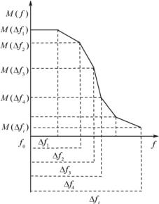
5.3 EMC Modeling Methodology |
139 |
Fig. 5.22 Spectrum distribution model near the fundamental wave of the transmitter
ponents in the transmitter, the time-domain characteristics of the radiation signal of the transmitter, the modulation method of the signal, the type of power amplification, and the filtering performance are different. As a result, the spectral power distribution of the transmitter is quite different from (5.71). The output power of the transmitter is not completely limited to a certain frequency or a narrow band, but is mainly distributed in the frequency band near the fundamental wave. In the process of EMC analysis and design, we need to know not only the spectrum power value within the frequency band of the transmitter, but also the out-of-band spurious and harmonic power values. The spectrum of the transmitter is described in [21].
The spectral distribution envelope near the fundamental frequency is described by a polyline segment. The power of each frequency point is determined by the maximum emission power of the fundamental wave, the frequency value of the point, and the position and slope of the polyline segment where the frequency point is located. The spectrum distribution model near the fundamental frequency of the transmitter is shown in Fig. 5.22.
Assuming that the central operating frequency of the transmitter at a certain moment is f0, the relative value of a certain spectral component and the maximum transmitting power of the fundamental wave is M( f ) (dBc), and then M( f ) can be expressed as
M( f ) |
|
M |
+ N |
lg( |
| f − f0| |
), ( f |
|
[ f |
i−1 |
, f |
]; i |
|
[1, n]) (5.74) |
|
|||||||||||||
|
i |
i |
|
fi |
|
i |
|
|
|||||
where fi is the frequency bandwidth between the low-end part of the i-th spectral component and the central operating frequency f0; Mi is the constant term of the

140 |
|
5 Critical Techniques of Quantitative System-Level EMC Design |
||||
Table 5.4 |
Harmonic |
|
|
|
|
|
|
Fundamental |
A |
B (dB) |
Standard |
||
suppression constants of |
|
|||||
|
frequency |
(dB/dec) |
|
deviation δ (dB) |
||
transmitters |
|
|
||||
|
(MHz) |
|
|
|
||
|
|
|
|
|
|
|
|
|
|
|
|
|
|
|
|
|
<30 |
−70 |
−20 |
10 |
|
|
|
30~300 |
−80 |
−30 |
15 |
|
|
|
>300 |
−60 |
−40 |
20 |
baseband modulation characteristic in the i-th frequency band; Ni is the slope of the spectral envelope within the frequency band [ fi−1, fi ],and it is a constant term; n represents the number of segments that the spectral envelope covers at the one side of the center frequency, and n ≥ 1. When n 0, the characteristics of the frequency spectrum can be simplified as (5.71).
According to Eq. (5.71), the spectrum power distribution near the fundamental wave of the transmitter is
P |
+ M( f ) |
(5.75) |
P( f ) ¯max |
|
|
¯
where Pmax is the statistical mean of the maximum radiation power of the transmitter. The spectral power of the harmonics can be statically calculated as
Ph |
(N |
h |
f |
) |
P |
+ A lg N |
h |
+ B |
(5.76) |
|
0 |
|
¯B |
|
|
|
¯
where PB is the statistical mean of the fundamental emission power; f0 is the fundamental frequency; Nh is the harmonic number; A, B are the harmonic suppression constants of the transmitter. For common transmitter, the value of A, B can be determined using Table 5.4.
Both Eqs. (5.74) and (5.76) are based on a large amount of priori data. They have a certain degree of universality, but the valuation bias is relatively large (as shown in Table 5.4). The prerequisite for using the two functions is that a large amount of test data has been obtained for the product. In addition, the functions only estimate the spectrum and harmonic power in the vicinity of the fundamental wave, but they are incapable of evaluating the out-of-band spurious power. In fact, if a mature product or similar system has already existed, we can directly test the full-band spectral power distribution data of the transmitting equipment and then substitute it into the EMC design.
In the engineering practice of EMC analysis and design, if the transmitter of the aircraft system is a mature product or an improved version of a mature product, we will use a test method similar to CE106 instead of (5.74) and (5.76) to measure the power distribution characteristics of the spectrum, which is denoted as Pt ( f ). Figure 5.23 shows the partial test data for the spectral power distribution of a transmitter. It is obvious that the spectral distribution shown in the figure is quite different from the spectrum distribution represented by Eqs. (5.74) and (5.76). Therefore,
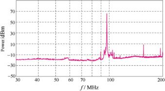
5.3 EMC Modeling Methodology |
141 |
Fig. 5.23 Partial test data of the spectral power distribution of a transmitter
when the spectral power distribution characteristics of the product can be obtained by testing, test data should be preferred; when the test data cannot be obtained, the results should be predicted first, and as soon as the test data can be obtained, the prediction results should be modified with the test data.
In the engineering practice of EMC analysis and design, if the transmitter selected for the aircraft system is a product to be developed, the maximum power value of the emission spectrum can be estimated using Eq. (5.77).
Pt ( f ) Psignal ( f ) · Gamp ( f ) · Pamp ( f ) · L f ilter · Pf ilter ( f ) |
(5.77) |
where Psignal ( f ) is the spectral power distribution of a weak signal input for a highpower microwave power amplifier of a transmitter. The signal’s characteristics in time domain can be simulated and calculated according to the circuit design scheme, and Psignal ( f ) can be obtained by a Fourier transform [19, 28]; Gamp ( f ) is the power gain of a high-power microwave power amplifier. It is a design input of the power amplifier which can also be provided by the product supplier. Pamp ( f ) is the spectral distribution characteristics of the power amplifier. For individual power amplifier components, the data can be measured before the development of the transmitter. Considering the nonlinear factor, the power amplifier should be in the maximum output state during the test. L is the attenuation of the emission power of the microwave filter; Pf ilter ( f ) is the spectral power distribution characteristic of the microwave filter.
For separate filter components, L f ilter and Pf ilter ( f ) can be provided by the product supplier or be tested before the development of the transmitter. Considering the nonlinear factors, the input power of the microwave filter needs to simulate the maximum output of the power amplifier. And for filters integrated into a specific circuit, these two data can be simulated and calculated during the design phase [28].
In-band and out-of-band radiation characteristics of airborne antennas. The radiation characteristics (directionality, direction power gain) of the airborne antenna
142 |
5 Critical Techniques of Quantitative System-Level EMC Design |
are important parts of the energy transmission from the transmitter to the susceptive port. The accuracy of this data has a great influence on the analysis and design of the system EMC.
When the antenna is installed on the surface of the fuselage, the boundary conditions formed by the installation environment of the antenna greatly affect the radiation characteristics of the antenna. The aircraft will induce electromagnetic current and generate secondary radiation, such that the radiation characteristics of the antenna will be remodeled.
In general, the radiation characteristics of the airborne antenna can be obtained by measurement or calculation. For small aircraft, if the antenna is installed and the test environment is available (in the darkroom), then the radiation characteristics of the airborne antenna can be obtained through measurement. For large and mediumsized aircraft, the test environment is difficult to build, and the design scheme for antennas is usually not fully determined during the demonstration phase. Therefore, the only way to obtain the radiation characteristics of the airborne antenna is through simulation calculations.
There is a large number of the research literatures on the radiation characteristics of structured antennas in free space, such as array antennas, horn antennas, parabolic antennas, and loop antennas, and relatively accurate calculation result has been achieved. After the installation, the antenna’s radiation characteristics are much more difficult to calculate. The major calculation methods are approximation and numerical methods. Our readers can refer to [10, 29–37] for more research under this topic.
Regarding the radiation characteristics of the antenna, we would like to point out in particular that the out-of-band characteristics of the antenna are nonnegligible in the study of EMC. In the traditional engineering development, only the in-band parameters such as power gain, pattern, characteristic impedance, and radiation efficiency are considered for the selection of the airborne antenna. In recent years, many problems have been found in the implementation of EMC engineering, which forced the engineers to pay more attention to the effects from the aircraft platforms on the antenna’s radiation characteristics. However, rare attentions have been paid to the out-of-band characteristics of antennas. In fact, the antenna at the front end of the equipment is equivalent to a filtering system, and its out-of-band response characteristics have an important influence on the out-of-band radiation characteristics of the transmitter and the out-of-band response of the receiver. There are plenty of transmitting and receiving antennas locating on the airborne platform, and the out-of-band of some antennas falls inside the in-band of other antennas. The out-of-band radiation characteristics of the antenna may cause mutual interference between the transmitting and receiving antennas. In practical applications, the authors have performed theoretical analysis and practical testing on the out-of-band characteristics of a large number of antennas. Generally, the antenna under study shows that: The directionality of the antenna may be split at the high frequency band, and the gain may become large. Although the radiation efficiency of the antenna is degraded, then the intensity of radiation is still relatively great, the energy transmitted by the transmitting antenna
5.3 EMC Modeling Methodology |
143 |
out-of-band can still cause interference to susceptive equipment, and the out-of-band of the susceptive equipment may also respond to the interference signal. In practical applications, the authors have incorporated the out-of-band characteristics of the antenna into the overall EMC design, which has significantly improved the accuracy of the EMC design [14].
(2)Receiver response model. The aircraft system is equipped with a large number of receiver for aeronautical navigation, detection, reconnaissance, warning, and communication. The normal operation of the receivers is of great significance for flight safety and performance, and it is also an important goal in aircraft EMC design. The receiver and its front-end antenna together constitute the response to electromagnetic energy in a specific spatial, polarization, time, and frequency domain. Among them, we mainly need to select the timedomain and the frequency-domain characteristics of the electromagnetic energy for the receiver. In the design of aircraft system EMC, the frequency-domain characteristics of the receiver are mainly considered.
For an ideal receiver, the frequency selectivity should exhibit a rectangular characteristic; i.e., the receiver is only susceptive to the electromagnetic energy in a specific frequency range, and all the energies outside the frequency range of the spectrum are rejected from entering the receiving channel. Due to the nonlinear effects of the functional circuits such as preselectors, mixers, filters, and IF amplifiers in receiver, the frequency selectivity and rectangular selection characteristics of the receiver are inconsistent. What’s more, the frequency selectivity and rectangular characteristics of some receivers are far from each other. In the EMC design process, the frequency selectivity of the receiver must be quantified.
Similar to the representation of the spectral distribution near the fundamental wave of the transmitter, the frequency selectivity of the receiver near the operating bandwidth or the major receiving channel can also be represented by a piecewise straight-line approximation [21].
S( f ) S( fi ) + Si lg( f / fi ) |
(5.78) |
where S( f ) is the selectivity of the receiving equipment when the frequency is
deviated from the tuned frequency as f ; S( |
fi ) is the value of the selectivity of |
|
the receiver on the frequency boundary |
fi ; Si |
is the slope of the selectivity of the |
receiver on the line segment of frequency |
fi . |
|
Signals located within the frequency points and frequency range outside the main receiving channel can also enter the receiver due to the system’s nonlinear characteristics, affecting the in-band of the receiving system. These frequencies or frequency bands are called additional receiving channels. They mainly include IF receiving channel, image receiving channel, and harmonic receiving channel. Using the same method, the selective model of the receiver in the main additional receiving channels
can be obtained |
|
S( fa ) I lg( fa / f0) + J |
(5.79) |
144 |
5 Critical Techniques of Quantitative System-Level EMC Design |
|||||
Table 5.5 Harmonic |
|
|
|
|
|
|
|
Frequency (MHz) |
I (dB/dec) |
J (dB) |
δ( fa ) (dB) |
||
suppression constants of |
|
|||||
<30 |
25 |
85 |
15 |
|||
transmitters |
||||||
|
30~300 |
35 |
85 |
15 |
||
|
|
|
|
|
|
|
|
>300 |
40 |
60 |
15 |
||
|
|
|
|
|
|
|
where f0 is the central operating frequency of the receiver; fa is the operating frequency of the additional receiving channel; I and J are linear approximation coefficients of the frequency selective curve.
¯
Selective models often use a statistical model, which exploits the mean S( fa ) and the mean squared error σ ( fn ), where I , J , and σ ( fn ) are obtained from data averaged over different types of receivers. Table 5.5 lists the mean of I ,J , and σ ( fn ) for different types of receivers.
Both Eqs. (5.78) and (5.79) are based on a large amount of priori data. They have a certain degree of universality, but the bias of the predicted value is relatively large (as shown in Table 5.5). The prerequisite for using the two functions is that a large amount of test data has been obtained for the product. Different types of receivers have different mechanisms when generating major additional channels, so the error in the estimation of additional channel selectivity may be greater using (5.79). If a mature product or similar system has already existed, we can also directly test the full-band selectivity data of the receiver and then substitute it into the EMC design. The accuracy of the analysis and evaluation will be improved in this way.
In a sense, the frequency range outside the working frequency band of the receiver (main receiving channel) can all be called additional receiving channels. Besides the IF receiving channel, the image receiving channel, and the harmonic receiving channel, if the input energy is large enough, the nonlinearity of the system may cause the receiver to respond to signals at any frequency outside the band. The fullband response characteristics of the receiver can be analyzed using the behavioral simulation method of the circuit [19, 28]. For mature equipment, it is best to use the test methods to accurately obtain the response characteristics: The sensitivity of the receiver can be measured by in-band method, and the intermodulation suppression characteristics of the testing receiver can be measured by out-of-band method.
(3)Energy coupling model. The coupling model mainly involves antenna coupling, field–line coupling, cable coupling, and aperture coupling.
Antenna coupling. A large number of transceiver antennas are installed within the limited space of the aircraft, and it is likely that these antennas are difficult to work together. The energy coupling between airborne transceivers of aircraft is one of the main ways for airborne receivers to be interfered. When performing EMC design and quantitative allocation of indicators, it is necessary to quantitatively analyze and control the energy of transmitting equipment coupled with the airborne receiving antenna through the antenna port.
5.3 EMC Modeling Methodology |
145 |
In the engineering design of EMC, when analyzing the coupling between the transmitting and receiving antennas, the electrical size, the shielding condition, the polarization state of the transmitting and receiving antennas, the operating frequency band, the out-of-band characteristics, and the mounting mode should be fully considered.
According to the different electrical sizes of the transmitting/receiving antennas, the coupling can be categorized into near-field coupling, far-field coupling, and nearfar mixing field. Among them, near-field coupling and near-far mixing field energy transfer can be solved by numerical methods such as moment method (MoM) and finite element method (FEM). When analyzing the coupling between antennas, we also need to consider whether there are obstacles between the antennas: For nearfield conditions, we can use low-frequency numerical methods no matter there are obstacles or not; for the far-field situation, if there is no obstacle, we can use the numerical method and the geometrical optics method to do hybrid analysis. The numerical method is used to calculate the radiation characteristics of the antenna, and the geometrical optics method is used to calculate the attenuation of the electromagnetic field in space. For cases where the transmitting and receiving antennas are in the far field of each other, and there is shielding between airborne antennas from the fuselage or the wing, we can use numerical method and geometrical theory of diffraction (GTD) or uniform geometrical theory of diffraction (UTD) to do hybrid analysis. The numerical method is used to calculate the radiation characteristics of the antenna, and GTD or UTD is used to calculate the attenuation, diffraction attenuation, and occlusion loss of the electromagnetic field in space.
The airborne antenna isolation is an indicator describing the antenna coupling. It fully reflects the directionality, gain, polarization state, in-band and out-of-band characteristics of the antenna, and the contribution of space between antennas to the energy coupling between transmitting and receiving antennas. Antenna isolation refers to the ratio of the transmitting power Pta of the transmitting antenna to the power Pra received by the receiving antenna (Pra is the power Pta received by the receiving antenna after various attenuations), i.e.,
L |
Pta |
or L(dB) 10 lg |
Pta |
(5.80) |
Pra |
Pra |
Antenna isolation is only one isolation item between the transmitter and the receiver. In engineering applications, although it is not possible to estimate the interference relationship between the transmitter and the receiver simply by the value of the antenna isolation, the antenna isolation analysis is the key technology in isolation of the transmitter and receiver.
In the following paragraphs, we will discuss the antenna isolation at far field without obstacle coupling, the antenna isolation at near-field coupling, and the antenna isolation at far field with obstacles coupling separately. Then, we will introduce the concept of isolation between transmitters and receivers.
(a)Antenna isolation at far field without obstacle coupling. Since the two antennas are far from each other, their energy coupling is mainly through the radiation

146 |
5 Critical Techniques of Quantitative System-Level EMC Design |
|
field. Assuming the transmitting power of the transmitting antenna is Pta , and |
|
the gain is Gt (θt , ϕt ); the receiving power of the receiving antenna is Pra , and |
|
the gain is Gr (θr , ϕr ); the distance between the receiving antenna and the trans- |
|
mitting antenna is D; normally, the antenna isolation can be solved by Eq. (5.80) |
|
when the transmitting/receiving antennas are in direct view. When the size of the |
|
transmitting/receiving antennas is relatively small, they can be approximately |
|
regarded as a point source with a certain directionality; thus, the electromag- |
|
netic wave transmitted by the transmitting antenna can be approximated as a |
|
spherical wave and further approximated to a plane wave at the position of the |
|
receiving antenna. The antenna isolation can be expressed as |
Lantenna (dB) Ld − Gt (θt , ϕt ) − Gr (θr , ϕr ) |
|
||
20 lg[ |
4π D |
] − Gt (θt , ϕt ) − Gr (θr , ϕr ) |
(5.81) |
λ |
|||
where Ld 20 lg[ 4πλD ] is the spatial isolation of the transmitting and the receiving antennas in direct view. It is determined by factors including the distance D between the transmitting and the receiving antennas and the analysis wavelength λ. Gt (θt , ϕt ) is the antenna gain of the transmitting antenna in the receiving direction, and it can be looked up from the radiation plot of the airborne transmitting antenna gain based on the relative positions of the antenna. The specific angle is determined by the position of the line-of-sight segment between the transmitting and the receiving antennas on the aircraft coordinate system. Gr (θr , ϕr ) is the antenna gain of the airborne receiving antenna in the transmitting direction. It can be looked up from the radiation plot of the airborne receiving antenna gain based on the relative positions of the antenna. The specific angle is determined by the position of the line-of-sight segment between the transmitting and the receiving antennas on the aircraft coordinate system.
When the polarization of the transmitting/receiving antennas does not completely match, we need to consider the loss L P caused by the mismatch polarization; i.e., the entire isolation of antennas is
Lantenna (dB) Ld − Gt (θt , ϕt ) − Gr (θr , ϕr ) + L P |
|
||
20lg |
4π D |
− Gt (θt , ϕt ) − Gr (θr , ϕr ) + L P |
(5.82) |
λ |
|||
Now, we will discuss the solution of the loss caused by the polarization mismatch. Assume the amplitude ratio of the orthogonal components Eθ and Eϕ of the transmitting polarized wave to be ρ1, and their phase difference is β1. Similarly, assume the amplitude ratio of the orthogonal components Eθ and Eϕ of the receiving polarized wave to be ρ2 and their phase difference to be β2. When the amplitude and phase of the two polarized waves are different, the loss of the polarization mismatch can be calculated as [38]
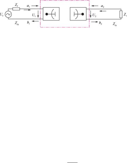
5.3 EMC Modeling Methodology |
147 |
Port 1 |
Port 2 |
Transmitting antenna |
Receiving antenna |
Fig. 5.24 Equivalent two-port network of near-field antenna coupling
L P 20 lg |
[1 + ρ1ρ2 cos(β1 + β2)]2 + [ρ1ρ2 sin(β1 |
+ β2)]2 |
|
|
|
(5.83) |
|
(1 + ρ1)2 + (1 + ρ2)2 |
|
||
When the magnitude of the two polarized waves is not identical, and β1 β2 0, the loss of polarization mismatch is
L P 20 lg |
(1 + ρ1ρ2)2 |
|
(1 + tgα1tgα2)2 |
(5.84) |
(1 + ρ1)2 + (1 + ρ2)2 |
(1 + tgα1)2 + (1 + tgα2)2 |
(b)Antenna isolation at near-field coupling. If the receiving antenna is not in the far-field region of the transmitting antenna or vice versa, the mutual interference between the two antennas does not couple with the radiation field but couples with the near-field bound field or the near-field induction field. This situation often occurs in isolation between the linear antenna arrays. Since the concept of antenna power gain is established in the far field, Eq. (5.80) does not apply to near-field antenna isolation analysis. Even if the concept of power gain is extended to the near field, it still describes the power gain of radiation field. However, in this case, the main factor of interference between antennas is not the radiation field.
In the near-field scenario, the system consisting of the transmitting/receiving antennas can generally be viewed as a two-port network as shown in Fig. 5.24. Assuming the maximum output power of the signal source to be Pt max and the power absorbed by the load impedance Zr to be Pr , then the antenna isolation is [3, 39, 40]
Lantenna |
Ptmax |
(5.85) |
Pr |
As shown in Fig. 5.24, the transmitter is equivalent to the signal source Ue, and its internal impedance is Ze; the receiver is equivalent to the load impedance Zr ; the radiating antenna and its port, and the receiving antenna and its port together constitute a two-port network, in which the Port 1 is connected to the transmitter through the transmission line with characteristic impedance Z0t and the Port 2 is connected to the receiver through the transmission line with characteristic impedance Z0r . Then, we introduce the normalized complex voltage inward waves a1 and a2, and outward waves b1 and b2. They are defined as
148 |
5 Critical Techniques of Quantitative System-Level EMC Design |
|||||||||||
|
a1 |
|
U1 + I1 Z0t |
|
|
|
||||||
|
|
2√ |
|
|
|
|
|
(5.86) |
||||
|
|
Z0t |
|
|
||||||||
|
a2 |
|
U2 + I2 Z0r |
|
|
|
||||||
|
|
2√ |
|
|
|
|
(5.87) |
|||||
|
|
Z0r |
|
|
||||||||
|
b |
|
|
U1 − I1 Z0t |
|
|
(5.88) |
|||||
|
|
|
|
|||||||||
|
|
1 |
|
2√ |
Z0t |
|
|
|
|
|||
|
b |
|
|
U2 − I2 Z0r |
|
|
(5.89) |
|||||
|
|
|
|
|
||||||||
|
|
2 |
|
2√ |
Z0r |
|
|
|
|
|||
Then, the normalized matrix S can be obtained as |
|
|||||||||||
|
b1 |
|
|
|
s11 s12 |
a1 |
(5.90) |
|||||
|
b2 |
|
|
s21 s22 |
a2 |
|||||||
The reflection coefficient of signal source impedance Ze relative to Z0t
as
1 Ze − Z0t
Ze + Z0t
The reflection coefficient of load impedance Zr relative to Z0r is
|
2 |
Zr − Z0r |
|
|||
|
||||||
|
|
Zr + Z0r |
||||
Then, we can obtain the power absorbed by the load as |
||||||
Pr |
1 |
|b2 |
|2 1 − | 2|2 |
|||
|
|
|||||
2 |
||||||
Assume the output power of the signal source is 21 |bs |2, where bs is
|
Ue/√ |
|
|
|
|
|
Ue |
|
|
|
bs |
Zot |
|
|
|||||||
|
Z0t |
|||||||||
Ze/Z0t + 1 |
Ze + Z0t |
|||||||||
The maximum output power of the signal source is |
|
|||||||||
|
P |
1 |
|
|
|bs |2 |
|
|
|||
|
2 1 − | 1|2 |
|
||||||||
|
tmax |
|
||||||||
Since a1 bs + 1b1, thus
is defined
(5.91)
(5.92)
(5.93)
(5.94)
(5.95)
bs a1 − 1b1 a1 − 1(s11a1 + s12a2) a1(1 − 1s11) − s12 1a2 (5.96)
Since b2 s21a1 + s22a2, a2 b2 2, thus

5.3 EMC Modeling Methodology |
149 |
L |
antenna |
|bs |2 |
|
|
|b2|2 1 − | 1|2 1 − | 2|2 |
|
|||
|
|
|||
|
|
|(1 − 1s11)(1 − 2s22) − s12s21 1 2|2 |
(5.97) |
|
|
|s12|2 1 − | 1|2 1 − | 2|2 |
|||
|
|
|||
In the near field, since the operating wavelength of the antenna is relatively long and does not satisfy the calculation conditions of the GTD, the antenna isolation in the near-field case can be calculated using (5.97). Using the FEM, the feed port of the transmitting/receiving antennas is used as the two ports of the two-port network. Then, the parameter S between the two can be calculated, and the VSWR of the antenna is calculated for each port. Substituting the parameters obtained by the numerical method into Eq. (5.97) will result in antenna isolation in the case of a near field.
When the FEM is used to calculate the antenna isolation, the optimization algorithm is used to calculate the matching impedance of the transmitting and receiving antenna ports. Thus, the impedance of the transmitting and the receiving antenna ports can be matched and we have 1 0, 2 0. Since the impedance matching has a frequency characteristic, when the operating frequency bands of the transmitting and the receiving antennas do not overlap with each other, 1 and 2 cannot equal to zero at the same time. In the emission frequency band, we have
L |
antenna |
|1 − 2s22|2 |
(5.98) |
|
|s12|2 1 − | 2|2 |
||||
|
|
In the receiving operating frequency band,
L |
antenna |
|1 − 1s11|2 |
(5.99) |
|
|s12|2 1 − | 1|2 |
||||
|
|
If the receiving and the transmitting bands are overlapped, then in the operating frequency band, there is
Lantenna |
1 |
(5.100) |
|s12|2 |
(c)Antenna isolation at far field with obstacle coupling. If the transmitting and the receiving antennas satisfy far-field area condition, and the fuselage or the wing is obstructed between the antennas, we then need to consider the attenuation or obstruction effect of the fuselage.
When there is diffraction, we can obtain the far-field antenna isolation according to (5.101).
Lantenna (dB) L P + Ld − Gt (θt , ϕt ) − Gr (θr , ϕr )

150 5 Critical Techniques of Quantitative System-Level EMC Design
L P + 20 lg[ |
4π D |
] + Ldi f f raction + S FW − Gt (θt , ϕt ) − Gr (θr , ϕr ) |
λ |
||
|
|
(5.101) |
where L P is the polarization attenuation between the transmitting and the receiving antennas; Ld is the spatial isolation between the transmitting and the receiving antennas; Ld is determined by the distance D between the transmitting and
the receiving antennas, the diffraction |
attenuation Ldi f f raction , the shielding atten- |
uation S FW , the analysis wavelength |
λ, etc. Therefore, Ld can be expressed as |
Ld 20 lg[ 4πλD ] + Ldi f f raction + S FW . Diffraction and block attenuation can be obtained by analyzing the surface diffraction or edge diffraction attenuation based on the diffraction model of the fuselage surface or the airfoil.
From the diffraction model, we can see that in order to obtain the diffraction attenuation of the field on the surface of the fuselage or the airfoil, it is necessary to accurately solve the trajectory of the diffraction ray. In the following paragraphs, we introduce a new algorithm for ray tracing “minimum included angle algorithm,” which was proposed by the EMC research team of Beihang University. This method improves the speed of tracing, the accuracy, and flexibility of calculation, and guarantees the uniqueness of ray tracing. This method can be used to perform calculation of ray tracing and isolation between any pair of antennas on the surface of the fuselage.
(d) Isolation between airborne transmitters and receivers. The ratio of the transmitting power Pt to the receiving power Pr is defined as the isolation between the transmitter and the receiver (where Pr refers to the power Pt that reaches the
receiver after various attenuations), i.e., |
Pt |
|
|
||
L |
Pt |
or L(dB) 10 lg |
(dB) |
(5.102) |
|
Pr |
Pr |
||||
|
|
|
|
|
|
Antenna isolation only takes into account the isolation between the transmitting and the receiving antennas and does not fully reflect the degree of isolation between the transmitter and the receiver. The factors affecting the energy transmission between the transmitter and the receiver are shown in Fig. 5.25. When analyzing the degree of isolation between a certain transmitter and a certain receiver, the frequency band attenuation of the transmitter, the loss of the transmission line, and the frequency band suppression characteristics of the receiver must be considered in addition to the isolation between the transmitting and the receiving antennas. Equation (5.103) is usually used for this analysis
LT R (dB) Lt B ( f ) + Lr B ( f ) + Lt f + Lr f + L P + Ld − Gt − Gr |
|
Lt B ( f ) + Lr B ( f ) + Lt f + Lr f + Lantenna |
(5.103) |
Equation (5.103) is the basis for the matrix elements of (5.95) and (5.62). From (5.103), it can be seen that antenna isolation is an important part of the isolation between the transmitter and the receiver. At the same time, the layout of the transmitting antenna has a relatively great impact on other susceptive ports, so the overall antenna layout design and optimization are quite important to the compatibility
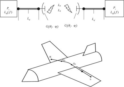
5.3 EMC Modeling Methodology |
|
151 |
|
Transmitter |
|
|
Receiver |
Transmission line |
|
Transmission line |
|
|
|
|
|
Transmitting |
Transmitting |
Receiving antenna Receiving |
Receiving |
input |
antenna Transmitting antenna |
antenna |
input |
port |
port |
port |
port |
Fig. 5.25 Factors influencing the isolation between the transmitter and the receiver
Fig. 5.26 Illustration of ray tracing on the surface
between the transmitter and the receiver. However, the antenna isolation is not completely equivalent to the isolation between the transmitter and the receiver, so other EMC indicators must be designed synergistically during the EMC design and optimization.
Constructing a three-dimensional geometric mesh model of the aircraft surface is an important basis for solving antenna isolation of airborne transmitters and receivers. Antenna coupling path is an important parameter in isolation calculation. When the mesh is dense enough, the computational cost to calculate the antenna coupling path will be very high, and it will be difficult even for a supercomputer to finish in a short time. Here, we will introduce the antenna coupling path calculation method based on the minimum included angle algorithm [41].
Calculating the coupling path between the transmitting and the receiving antennas on an arbitrary surface is essentially solving the problem with a geodesic [42]. In a well-defined area of the curve, there is only one curve between the two points to ensure that the path length is the minimum. This particular curve is called a geodesic. The creeping wave travels along the surface of the curved surface and can be seen as a geometric optical ray. Its propagation satisfies Fermat’s principle that the path of propagation is the shortest. As shown in Fig. 5.26, the path of the surface ray between the two points of Q1 and Q2 is the geodesic connecting the two points. Q1 is the point of tangency of the ray SQ1 on the surface of the aircraft, and the point Q2 is the point of tangency of the ray SQ2 on the surface of the aircraft.

152 |
5 Critical Techniques of Quantitative System-Level EMC Design |
Fig. 5.27 Mesh subdivision of the model surface
In order to track the surface rays, it is assumed that [43]: The creeping wave inside a single triangle is a straight line; when two adjacent triangles develop into a plane, the creeping wave trajectories on the two triangles are a straight line when connected.
Any surface can be split into multiple triangular planes, as shown in Fig. 5.27, and the coordinates of the vertices of each triangle can be obtained. Taking vertex
(B) and all the triangles that contain vertex (B), as shown in Fig. 5.28, v is the vector from the source point to the destination point. Starting from point B, the triangular edge BCi which forms the smallest angle with v is the creeping track we are looking for. In Fig. 5.28, assuming that the angle between BC2 and v is the smallest, the wave propagates along BC2. Then, with C2 as the new vertex, the creeping wave propagation trajectory is found using the principle of minimum included angle, and so on. With the minimum included angle method, we only need to analyze and compare the triangular edges within a certain range in the direction of v in the tracking process, which greatly improves the tracking efficiency. The included angle
formula is: |
→ |
→ |
→ |
|
→ |
|
|
· |
|
||||
θ min{θ1, θ2, θ3} min{arccos( |
υ |
· BCi /( |
υ |
BCi ))} |
(5.104) |
|
|
|
Curve 1 in Fig. 5.29 can be obtained as a sawtooth waveform using the minimum included angle method. On this basis, a NURBS curve [44] is constructed. The
rational fractional expression of the NURBS curve is:
n
k 0 ωk pk Bk,d (u) (5.105)
n
k 0 ωk Bk,d (u)
where pk is the n + 1-th control point; the parameter ωk is the weighting factor of the control point; the larger the ωk , the closer the curve is to the control point pk ; Bk,d (u) is the basis function of the B-spline function; it is defined as
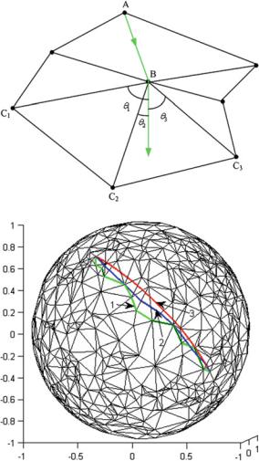
5.3 EMC Modeling Methodology |
153 |
Fig. 5.28 Illustration of the algorithm based on the triangle mesh
Fig. 5.29 Ray tracing process
Bk,d (u) 1, uk ≤ u ≤ uk+1 (5.106) 0, other
Therefore, as long as the control point, the weighting factor and the weight vector are extracted from the sawtooth wave Curve 1, and a NURBS curve can be defined. The NURBS curve can be further interpolated and fitted. The interpolation fitting method is to compare the curvature of the NURBS curve at each pre-interpolation point with the given radius of curvature threshold Rmax : If Ri < Rmax , it indicates that the curvature of the interval is large and it is suitable to use the arc segment fitting; if Ri > Rmax , it indicates that the bending degree of this interval is small. Based on
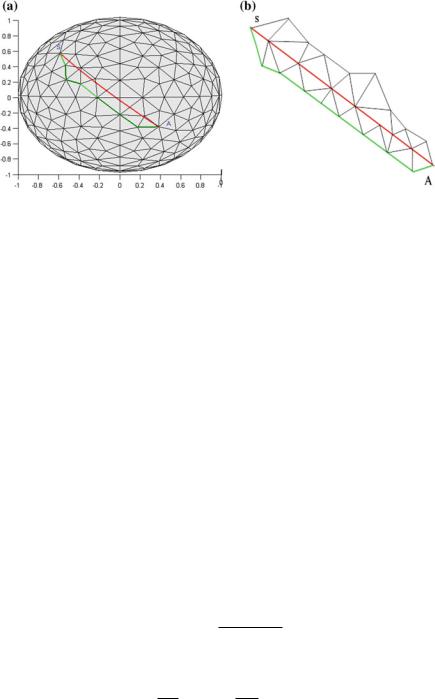
154 |
5 Critical Techniques of Quantitative System-Level EMC Design |
Fig. 5.30 Convergence of minimum included angle ray tracing. a Ray tracing on sphere and b projection of sawtooth wave on a plane
this idea, only the triangles near Curve 1 are more densely divided to obtain the Curve 2 in Fig. 5.29. Then, we keep interpolating using the same method until a two-dimensional smooth Curve 3 in Fig. 5.29 is formed. Therefore, the computing time can be greatly saved using the minimum included angle algorithm.
In the tracking process, the wave follows the direction which forms the smallest angle with the direction vector v, as shown in Fig. 5.30a. Therefore, a sawtooth wave that is creeping along the direction vector v is obtained on the curved surface. When the sawtooth wave is projected on the plane of the direction vector and perpendicular to the plane of the tracking ray and the direction vector v (Fig. 5.30b), the included angle will be the smallest, such that the sawtooth wave is guaranteed to connect to the endpoint A, which ensures it convergence.
In order to verify the accuracy and versatility of the algorithm, the algorithm was applied to developable surfaces and nondevelopable surfaces, respectively. The accuracy of the algorithm was verified by comparing the programmed trace results with the numerical results. Considering the direct wave and creeping wave, according to the new algorithm, the ray tracing path between the left and right of the cylinder can be obtained as shown in Fig. 5.31.
The geodesic line from the emission point S to the receiving point R satisfies Fermat’s principle. The tracing rays are divided into three segments: RP1, P1P2, and SP2. RP1 and SP2 can be viewed as direct waves on a concave surface. P1P2 is the creeping waves on the cylinder, as shown in Fig. 5.32. The geodesic on the cylinder can be calculated by the following formula
| P1 P2| h2 + | P2 Q|2 |
(5.107) |
Therefore, the numerical calculation length is
L S P2 + P1 P2 + P1 R 5.284
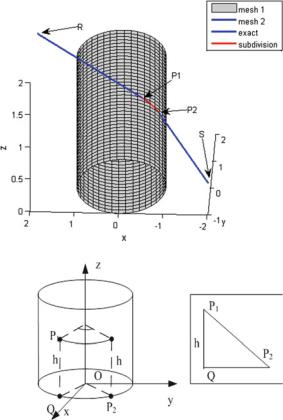
5.3 EMC Modeling Methodology |
155 |
Fig. 5.31 Ray tracing between two sides of the cylinder
Fig. 5.32 Calculation of the geodesic line on the cylinder
Table 5.6 Comparison of calculation results and tracing results on arbitrary surfaces
Coordinates of the |
Coordinates |
Coordinates |
Coordinates |
Tracing |
Numerical |
emission point S (m) |
of the |
of the point |
of the point |
result (m) |
distance |
|
receiving |
of tangency |
of tangency |
|
(m) |
|
point R (m) |
(P1) (m) |
(P2) (m) |
|
|
|
|
|
|
|
|
2 |
−2 |
0.511 |
−0.973 |
5.245 |
5.284 |
2 |
−1 |
0.860 |
−0.231 |
|
|
1.5 |
0.5 |
1.163 |
0.750 |
|
|
|
|
|
|
|
|
The numerical calculation results can then be compared with the tracing results, as listed in Table 5.6.
Using the new algorithm, the relative error between the tracing result and the ground truth is: a (5.284 − 5.245)/5.245 0.74%. It can be seen that the minimum included angle method is very accurate in result tracing on the developable surface, so the algorithm is applicable to the developable surface.
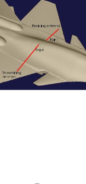
156 |
5 Critical Techniques of Quantitative System-Level EMC Design |
Fig. 5.33 Reflection and ray tracing of EM wave on the wing
The reflection and ray tracing of EM wave on the convex–concave surface: Reflected waves are also one of the factors that affect antenna isolation. A simple model is constructed for the reflected waves as shown in Fig. 5.33. The transmitting antenna on the left plane emits a wave, which is reflected by the left plane and directly hits the cylinder. After creeping on the cylinder for a certain distance, the reflection occurs on the right plane and then arrives at the receiving antenna.
As can be seen from Fig. 5.33, after importing the model into the program, the geodesic reflection from the transmitting antenna to the receiving antenna can be obtained. Therefore, the minimum included angle method is suitable for convex— concave surfaces.
Ray tracing on nondevelopable surfaces: Taking an ellipsoid as an example, we will illustrate that the minimum included angle method can be applied to the solution of a geodesic line on a nondevelopable surface. Taking two points at the end of the x- axis, according to the algorithm, the ray tracing path on the ellipsoid can be obtained, as shown in Fig. 5.34.
The approximation of the circumference of an ellipse is
L ≈ π 1.5(a + b) − |
√ |
(5.108) |
ab |
Table 5.7 compares the numerical result with the tracing result.
Using the new algorithm, the relative error between the tracking result and the ground truth is: a (13.4015 − 13.1534)/1.4015 0.36%. It can be seen that the
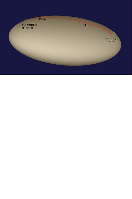
5.3 EMC Modeling Methodology |
157 |
Fig. 5.34 Ray tracing on the ellipsoid
Table 5.7 Comparison between numerical result and tracing result on the ellipsoid
Coordinate of the |
Coordinate of the |
Tracing result (m) |
Numerical distance |
emission point S (m) |
receiving point R (m) |
|
(m) |
|
|
|
|
−6 |
6 |
13.3534 |
13.4015 |
0 |
0 |
|
|
|
|
|
|
0 |
0 |
|
|
|
|
|
|
tracing result is very accurate. Therefore, the minimum included angle method is applicable to nondevelopable surfaces.
Ray tracing on a combination of solids: We use a combination of cone and cylinder to verify that the algorithm is also feasible for combination of solids. The lateral surface of the cone is a circular sector (SBC), as shown in Fig. 5.35. Thus, we can calculate the length of the geodesic line between any two points on the cone using Eq. (5.109)
B D2 B S2 + S D2 − 2B S S D cos θ |
(5.109) |
The ray path on the combination of solids as shown in Fig. 5.36 can be obtained using the algorithm. The ray path includes SD on the cone and DR on the cylinder.
So, the length calculated numerically is
L S D + D R 5.942
Table 5.8 compares the numerical result with the tracing result.
158 |
5 Critical Techniques of Quantitative System-Level EMC Design |
Fig. 5.35 Lateral surface of the cone
Fig. 5.36 Ray tracing on a combination of solids
Table 5.8 Comparison between numerical result and tracing result on a combination of solids
Emission point S (m) |
Receiving |
Inflection |
Emission |
Tracing |
Numerical |
|
point R (m) |
point D (m) |
point S (m) |
result (m) |
distance |
|
|
|
|
|
(m) |
|
|
|
|
|
|
0.489 |
0.996 |
0.85 |
0.489 |
5.942 |
5.897 |
|
|
|
|
|
|
−0.49 |
0.091 |
−0.481 |
−0.49 |
|
|
2.308 |
0.689 |
1.997 |
2.308 |
|
|
|
|
|
|
|
|
Using the new algorithm, the relative error between the tracking result and the ground truth is: a (5.942 − 5.897)/5.897 0.76%. It can be seen that the tracing result is very accurate, such that the minimum included angle method is applicable to assemblies. Figure 5.37 shows the result for an aircraft obtained from the ray tracing.
Result analysis: During tracing, the surface of the model is split into triangles. Therefore, the geodesic line obtained using the minimum included angle method is

5.3 EMC Modeling Methodology |
159 |
Fig. 5.37 Ray tracing result of an aircraft
Fig. 5.38 Tracing result analysis
not a smooth curve. In fact, the geodesic line is composed of three segments, which are a, b, and c in Fig. 5.38, i.e.,
L a + b + c |
(5.110) |
However, the actual length of geodesic line is the arc length:
S R L1 + L2 + L3 |
(5.111) |
It can be seen that the length of the geodesic line obtained by the new algorithm is very different from the ground truth. The error of the ray tracing is mainly determined by the density of the curved surface. The denser the split, the more accurate the result, and the more computing time it takes.
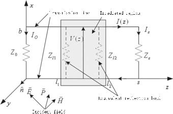
160 |
5 Critical Techniques of Quantitative System-Level EMC Design |
Fig. 5.39 Transmission line radiated by electromagnetic fields and the equivalent parameter settings
Field–line coupling. The electromagnetic field radiated by the aircraft’s airborne transmitters may affect the susceptive equipment through antenna coupling and cable coupling. Besides the distribution of the space, the coupling of the cable to the space field is also affected by the laying mode, the connection mode (such as single-wire grounding, double-line reciprocation), and the protection mode (unshielded single wire, single-shielded single wire, double-shielded single wire, twisted pair, shielded twisted pair, etc.) of the cables.
The connection between equipment often uses parallel two-conductor lines. Let the length of the parallel two-conductor lines be l, the spacing be b, and the height from the reference ground be h. The transmission line is exposed to the electromagnetic field as shown in Fig. 5.39. The area of the transmission line being exposed is A1, and then
|
∂ |
|
|
( × E) · nd S − |
|
B · nd S |
(5.112) |
∂t |
A1
There is an induced voltage for a given transmission line impedance, which is
b |
|
V (z) − Ex (x, z)dx |
(5.113) |
0 |
|
Then, we can derive the differential equations for the transmission line as [23, 45]

5.3 EMC Modeling Methodology |
|
161 |
||||||
|
|
∂ V (z) |
b |
|
||||
|
|
Byi (x, z)dx |
|
|||||
|
|
|
|
|
+ Z I (z) jω |
(5.114) |
||
|
|
∂ z |
|
|||||
|
|
|
|
|
|
0 |
|
|
∂ I (z) |
|
|
b |
|
||||
+ Y V (z) jωY |
Exi (x, z)dx |
(5.115) |
||||||
|
|
|
|
|||||
|
|
∂ z |
||||||
|
|
|
|
|
|
0 |
|
|
where Ei and Bi are incident field; Y and Z are the admittance and impedance of the transmission line, respectively.
If the equivalent impedance Z0 of the transmission line shown in Fig. 5.39 is not affected by the electromagnetic field, and the load of the transmission line is Zs , then the currents through Z0 and Zs that can be calculated using (5.114) and (5.115) are
I0 ZC
D[ZC cosh(γ l1) − Zl1 sinh(γ l1)]
l2
·[Ezi (b, z) − Ezi (0, z)][Zc cosh γ (l2 − z) + Zl2 sinh γ (l2 − z)]dz
l1 |
|
|
|
|
b |
b |
|
+ [ZC cos γ (l2 − l1) + Zl2 sinh γ (l2 − l1)] Exi (x, l1)dx − ZC |
Exi (x, l2)dx |
||
|
0 |
|
0 |
Is |
ZC |
|
(5.116) |
|
|||
D[ZC cosh(s − l2) + Zl2 sinh γ (s − l2)] |
|
||
|
l2 |
|
|
·[Ezi (b, z) − Ezi (0, z)][Zc cosh γ (z − l1) + Zl1 sinh γ (z − l1)]dz
l1 |
|
b |
b |
− [ZC cosh(γ l2) + Zl1 sinh(γ l2)] Exi (x, l2)dx + ZC |
Exi (x, l1)dx |
0 |
0 |
|
(5.117) |
where ZC is the characteristic impedance of the transmission line; γ is the complex propagation constant; b is the line spacing; s is the total length of the transmission line; l1 and l2 are the positions of the electromagnetic radiation transmission line. And there is
D (ZC Zl1 + Zl2 ZC ) cosh γ (l2 − l1) + (ZC2 + Zl2 Zl1) sinh γ (l2 − l1) (5.118)
where Zl1 and Zl2 are equivalent reflection loads at l1 and l2, which can be written as
Z |
l1 |
|
Z |
|
Z0 − ZC tanh γ l1 |
(5.119) |
|
C ZC − Z0 tanh γ l1 |
|||||||
|
|
|
|||||
162 |
5 |
Critical Techniques of Quantitative System-Level EMC Design |
|||||
|
Z |
l2 |
|
Z |
|
Zs + ZC tanh γ (s − l2) |
(5.120) |
|
C ZC + Zs tanh γ (s − l2) |
||||||
|
|
|
|
||||
Equations (5.116) and (5.117) are the induced currents obtained by irradiating an electromagnetic field to a certain area. For cases where multiple areas on the transmission line are irradiated, the superposition method can be used to solve the problem.
Because all the cables laying on the aircraft are affected by the distribution of the space field, the workload of analysis and calculation is huge, such that the influence is difficult to be fully predicted during predesign. To solve this problem, we can exploit the knowledge of engineering development, test, and usage of other similar equipment, to screen, forecast, and calculate the key parts of the cable.
Aperture coupling. There are many high-power transmitters and susceptive equipment in the cabins of aircraft systems. For susceptive equipment, it is required that the enclosures have good shielding capabilities. In fact, many pieces of susceptive equipment have to include apertures of different sizes and numbers; thus, the electromagnetic field in the cabin can be coupled with the apertures and acts on the cables and susceptive components inside the casing of the equipment. At the same time, the high-power radiation field outside the fuselage can also be coupled with the inside of the fuselage through apertures, thereby affecting the environment electromagnetic fields, cables, and equipment inside the cabin.
The analysis of the aperture-coupled electromagnetic field is complex, and it is difficult to obtain an accurate analytical solution. Generally, diffraction theory or electromagnetic dual theory is used to obtain approximate results [46].
The theoretical basis for diffraction in physical optics is the Huygens principle, which assumes that every point on the wave front can be seen as a secondary light source that radiates wavelets. The wavelets are then stacked in front of the transmission direction; thus, the field quantity in the transmission direction can be obtained. Based on Huygens principle and the Kirchhoff formula derived from Green’s theorem, the field quantity ψ (r) (omitting the time factor e−jωt ) at any point P in a certain area V after the aperture coupling can be expressed as ψ and ∂∂ψn of the boundary surface S from V as
|
1 |
|
e− jk R |
|
|
1 |
|
R |
|
|
ψ (r) − |
|
|
|
n ψ + |
jk − |
|
|
|
ψ d S |
(5.121) |
4π |
|
R |
R |
K |
||||||
S
where R is the distance from the field point (P) to the center of the aperture.
The center of the aperture is set to be the origin of the Cartesian coordinate system. The field intensity at the center of the aperture is ψ0. The incident wave is projected onto the conductive plate at an angle θ0. The angle between the radius vector from the field point to the center of the aperture and the normal direction of the conductive plate is θ . For apertures of any shapes, we have
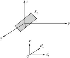
5.3 EMC Modeling Methodology |
163 |
Fig. 5.40 Rectangle aperture coupling
ψ (r) j |
ke− jk R |
(θ0 + θ ) ψ0e− jkr d S |
(5.122) |
4π |
|||
|
|
S0 |
|
For a rectangle aperture S0 as shown in Fig. 5.40, let the length of the aperture be 2a, and the width be 2b. The incident ray is along the direction of z-axis and θ0 00. The incident field is Ey E0e− jkr ; thus, there is a coupling field and we have
EP − |
jke− jk R |
(1 + cosθ ) |
e− jkr d S |
|
4π R |
|
|||
|
|
|
S0 |
|
− |
jke− jk R |
(1 + cosθ ) |
E0e− jk(x si n θ cosϕ+y si n θ si n ϕ)dx dy |
(5.223) |
4π R |
||||
|
|
|
S0 |
|
where R is the distance from the field point to the origin; θ is the angle between R and the z-axis; E0 is the field strength of the incident wave at the rectangle aperture plane S0; ϕ is the angle between the projection of R on xoy and the x-axis; x , y are the coordinates of any point on the rectangle aperture plane S0.
For circular aperture S0 as shown in Fig. 5.41, let the aperture radius be a. When the incident field is a constant, i.e., Ey E0, the coupling field is
EP − |
jke− jk R |
E0 S(1 + cosθ ) |
2 J1(ka sinθ ) |
(5.124) |
4π R |
ka sinθ |
where J1 is a first-order Bessel function and S π a2.
In addition, when the conductive plate is thin, and the size of the aperture is small compared to the wavelength, the distribution of the aperture coupling field can be approximated using the electromagnetic dual principle.
Coupling between cables. Due to space limitations, large number of equipment, and difficulty in equipment layout adjustment, the internal cables of the aircraft

164 |
5 Critical Techniques of Quantitative System-Level EMC Design |
Fig. 5.41 Circular aperture coupling
are densely populated. Sometimes, high-power RF cable accessories are installed with a large number of weak signal transmission cables. In this situation, mutual coupling between cables may cause interference response or decrease of safety margins of the susceptive equipment.
Cable coupling can be capacitive or inductive. There are many kinds of coupled cables, such as unshielded line coupling, shielded line coupling, unshielded twisted pair coupling, and shielded twisted pair coupling. Among them, the radiation coupling relationship between two parallel wires located above the ground plane is very typical (the height from the ground, the radius of the insulation layer, and the radius of the wire layers of the two wires are referred to as h1, R1, r1 and h2, R2, r2 respectively; the distance between the two wires is denoted by s; the length of the two parallel wires is denoted by ls ; the dielectric constant of the insulating layer is denoted by ε).
The equivalent distributed parameters of the capacitive coupling between the radiating cable and the receiving cable are shown in Fig. 5.42. The coupling capacitance between the two parallel wires is
|
|
|
|
C12 |
− |
|
|
2π εe f f |
P12 |
|
|
|
|
(5.125) |
||||||||
|
|
|
|
cosh−1 |
h1 |
− |
cosh−1 |
h2 |
P2 |
|||||||||||||
|
|
|
|
|
|
|
|
|
|
r1 |
|
|
|
r2 |
12 |
|
|
|
|
|
||
P |
|
1/2 cosh−1 |
s2 + (r12 − r22) |
|
+ cosh−1 |
|
s2 − (r12 − r22) |
|
|
|
|
|||||||||||
|
|
|
|
|
|
|
|
|||||||||||||||
12 |
|
|
|
|
2sr1 |
|
|
|
|
|
2sr2 |
|
|
|
|
|||||||
|
− |
cosh−1 |
4h1h2 + s2 + (r12 − r22) |
− |
cosh−1 |
|
4h1h2 + s2 − (r12 − r22) |
|
||||||||||||||
|
|
|
|
|
|
|
||||||||||||||||
|
|
2r1 |
|
4h1h2 + s2 |
|
|
|
|
|
|
2r2 |
4h1h2 + s2 |
||||||||||
(5.126)
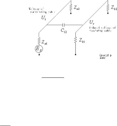
5.3 EMC Modeling Methodology |
165 |
Fig. 5.42 Equivalent distributed parameters of capacitive coupling of parallel laying between radiating and receiving cables
R1 +R2 2 − 1
r1 +r2
εe f f ε0 + 2 2 (ε − ε0) (5.127)
2s+R1 +R2 r1 +r2
The equivalent capacity of capacitive coupling of parallel laying between radiating and receiving cables can be used to solve the coupling voltage, i.e.,
U2 |
|
1 |
|
U1 |
(5.128) |
1 + |
1 |
|
|||
jω ZC12ls |
|
|
|||
|
|
|
|
||
where Z Zb1 Zb2 .
Zb1 +Zb2
If the radiating cable is a shielded cable, let te be the thickness of the shielding layer, δe be the skin depth of the emitting shielding line, rsi be the radius of the inner conductor of the shielding layer, and Fe be the constant related to the coverage of the shielding layer. Then, we have
|
|
|
|
|
1 |
|
e− |
te |
|
1 |
|
|
|
|
|
|
U2 |
|
|
|
δe |
+ Fe |
|
|
|
U1 |
(5.129) |
||||
1 + |
1 |
|
1 + |
|
1 |
|
|||||||||
jω ZC12ls |
|
|
|
jω Rs Cws ls |
|
|
|||||||||
|
|
|
|
|
|
|
|
|
|
|
|||||
where Cws |
2π ε |
is the capacitance value between the core and shielding layer |
|||||||||||||
ln(rsi /r1 ) |
|
||||||||||||||
of the radiating wire per unit length; Rs is the shielding resistance which depends on frequency. The expression of Rs is
|
te |
|
sinh |
2te |
+ sin |
2te |
|
Rs R0 |
|
δe |
δe |
||||
δ |
e |
cosh |
2te |
− cos |
2te |
||
|
|
δe |
δe |
||||
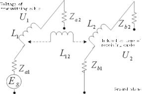
166 |
5 Critical Techniques of Quantitative System-Level EMC Design |
Fig. 5.43 Equivalent distributed parameters of inductive coupling of parallel laying between radiating and receiving cables
where R0 |
|
les |
is the DC resistance of the shielding layer, les |
is the length of |
|||||||||||||||
|
2π σ rsi t |
||||||||||||||||||
the shielding wire, σ is the electric conductivity of the shielding layer, and t |
is the |
||||||||||||||||||
thickness of the shielding layer. |
|
|
|
|
|
|
|
|
|
|
|
||||||||
For double-shielded radiation cables, there is |
|
|
|
|
|
|
|
||||||||||||
|
|
|
|
|
|
|
te |
|
|
|
|
|
te2 |
|
|
|
|
|
|
|
|
|
1 |
|
e− |
1 |
|
|
e− δe2 + Fe2 |
1 |
|
|
|||||||
U2 |
|
|
|
δe |
+ Fe |
|
|
|
|
U1 |
|||||||||
|
|
1 |
|
1 |
|
|
1 |
|
|||||||||||
1 + |
|
|
|
|
|
1 + |
|
|
|
|
1 + |
|
|
|
|||||
jω ZC12ls |
|
|
|
jω Rs Cws ls |
jω Rs2Cs1s2ls |
|
|||||||||||||
|
|
|
|
|
|
|
|
|
|
|
|
|
|
|
|
|
(5.130) |
||
where Cs1s2 is the capacitance value between the inner and outer shielding layers per unit length; Rs2, te2, δe2, and Fe2 are the impedance, thickness, skin depth, and shielding constant of the outer shielding layer, respectively.
The equivalent distributed parameters of the inductive coupling between the radiating cable and the receiving cable are shown in Fig. 5.43. The mutual inductance between parallel cables is
L12 |
μ0 |
(h1 + h2)2 + s2 |
(5.131) |
|
|
ln |
|
||
4π |
(h1 − h2)2 + s2 |
|||
The induced voltage of the receiving cable due to the inductive coupling at the
terminal load Zb2 is |
|
|
|
|
|||
|
|
|
|
UL |
jωL12 I1ls |
Zb2 |
(5.132) |
|
|
|
|
Zb1 + Zb2 + jωL2ls |
|||
where L2 |
μ0 |
ln |
2h2 |
− 1 |
; I1 is the radiating cable current; L2 is the self-inductance |
||
2π |
r2 |
||||||
per unit length of the receiving cable. The expression for current I1 is
5.3 EMC Modeling Methodology |
|
167 |
I1 |
U1 |
(5.133) |
|
||
Za2 + jωL1ls |
where U1 is the voltage of the radiating cable; L1 is the self-inductance per unit length of the radiating cable, and its expression is
L1 |
μ0 |
2h1 |
− 1 |
(5.134) |
|
|
ln |
|
|||
2π |
r1 |
||||
If the radiating cable is shielded and grounded at multiple points, the radius of the shield is rs , the self-inductance per unit length of the shield is Lsw, the resistance of the radiating cable shield is Rs , and the induced voltage of the shield is Us , then the induced current of the shield can be calculated as
|
Us |
|
|
jωLsw I1ls |
|
|
jω I1ls |
μ0 |
ln( |
2h1 |
− 1) |
||||||
Ish |
|
|
|
|
2π |
rs |
|
||||||||||
|
|
|
|
|
|
|
|
|
|
|
|
|
|
(5.135) |
|||
Rs + jωLswls |
|
Rs + jωLswls |
Rs + jωLswls |
μ0 |
|
ln( |
2h1 |
|
|
||||||||
|
|
|
|
|
|
|
|
2π |
|
rs |
− 1) |
||||||
Correspondingly, the equivalent radiation inference is |
|
|
|
|
|
|
|
|
|||||||||
Ie f f I1 − Ish |
|
|
Rs I1 |
|
|
|
Rs I1 |
|
|
|
|
|
(5.136) |
||||
|
|
|
|
|
|
|
|
|
|||||||||
Rs + jωLswls |
Rs + jωls |
μ0 |
2h1 |
|
|
|
|||||||||||
|
|
|
|
|
|
|
2π ln( |
rs |
− 1) |
||||||||
The induced voltage of the receiving cable due to the inductive coupling to the
terminal load Zb2 is |
|
|
|
|
|
|
|
|
|
|
||
UL jωL12 Ie f f ls |
Zb2 |
|
|
|
|
|
|
|
|
|
|
|
Zb1 + Zb2 + jωLswls |
|
|
|
|
|
|
|
|||||
jωL12ls |
|
Zb2 |
|
|
|
|
|
Rs I1 |
|
|
||
Zb1 + Zb2 + jωls |
μ0 |
ln( |
2h1 |
− 1) |
|
μ0 |
ln( |
2h1 |
− 1) |
|||
|
2π |
|
rs |
|
Rs + jωls 2π |
rs |
||||||
(5.137)
If the receiving cable is shielded and grounded at multiple points, Ls2w2 is the mutual inductance between the shielding layer and the receiving core per unit length, Rrs is the resistance of the receiving cable’s shielding layer, Les2 is the mutual inductance between the radiation cable and the receiving cable’s shielding layer per unit length, Lew2 is the mutual inductance between the radiating cable and the receiving cable per unit length, Lrs is the self-inductance of the receiving cable shielding layer per unit length, and U2 is the induced voltage of the receiving cable core, then the induced current and the induced voltage of the shielding layer are
Irs |
Urs |
|
jωLes2ls I1 |
(5.138) |
Rrs + jωLrsls |
Rrs + jωLrs ls |
168 5 Critical Techniques of Quantitative System-Level EMC Design
U2 jωLew2ls I1 − jωLs2w2ls Irs jωLew2ls I1 − jωLs2w2ls jωLes2ls I1
Rrs + jωLrsls
(5.139)
5.3.2.3Nonlinear System Behavioral Modeling Method
In the system-level EMC study, it is necessary to build a behavioral model of the nonlinear system in order to analyze the nonlinear factors that affect the characteristics of the system. On this basis, we need to linearize the nonlinear subsystems and equipment, and improve the accuracy of the equipment’s EMC behavioral simulation modeling.
This book takes the power amplifier, a most common nonlinear device in communication systems, as an example to explain the modeling process. The nonlinear description method is used to establish a behavioral model of the nonlinear system. With this method, we can further study the spectrum regeneration or expansion outside the useful signal bandwidth among the communication systems, and the mutual interference between adjacent channels [16].
1. The nonlinearity of electronic systems
Nonlinearity in electronic systems is mainly reflected in the following aspects.
(1) The generation of harmonics
One of the most obvious characteristics of a nonlinear system is the generation of harmonics of the excitation frequency. If a nonlinear system is represented by a Taylor series expansion, when the input is a single-frequency signal u(t) A cos ω1t, the output contains not only the fundamental frequency component but also the harmonic component at frequency N ω1 (where N is a positive integer), as shown in Fig. 5.44. In most cases, the harmonics can be filtered out in narrowband receiving systems, but in the broadband system, the harmonics may cause serious interference to the system. All amplifiers will produce harmonics of different strengths. The stronger the harmonics, the worse the nonlinearity of the amplifier is.
(2) Intermodulation
Intermodulation is the recombination of several frequencies. When the input is a dual-tone signal, the output frequency can be expressed as mω1 + nω2 (m, n
· · · , −3, −2, −1, 0, 1, 2, 3, · · ·). The intermodulation can cause serious interference
Non-linear system
Fig. 5.44 Input and output spectrum diagram of a single signal through the nonlinear system
5.3 EMC Modeling Methodology |
169 |
to the receiver. The intermodulation caused by the third power term of the nonlinear device is called the third-order intermodulation, and the intermodulation caused by the fifth power term is called the fifth-order intermodulation. The third-order intermodulation signal is the strongest signal in the odd-order terms. When the frequencies of the two input signals are very close, the third-order intermodulation signal is difficult to filter out.
(3) Cross-modulation
Cross-modulation is also caused by the nonlinearity. When the modulation of one signal is converted into another signal, it will result in cross-modulation distortion, which is likely to interfere with the adjacent channels.
(4) Saturation and dynamic range reduction
When the power amplifier operates in the nonlinear region, the response current does not increase proportionally with the increase of the excitation voltage. Under certain conditions, the amplifier saturates, and the amplification factor and the dynamic range of the amplifier decrease, making the amplifier unable to meet the design requirements. The power consumption will also be increased in the same time.
(5) Conversion of amplitude modulation/phase modulation (AM/PM)
AM–PM conversion refers to the phase deviation caused by the change of signal amplitude in a nonlinear circuit. In RF power amplifiers, phase distortion can also cause the third-order intermodulation distortion.
2. Nonlinear system modeling
In system-level EMC studies, amplifier (including power amplifier) is a common and important electronic device of all electronic systems. The amplifier’s inherent nonlinearity usually leads to spectrum regeneration or expansion outside the useful signal bandwidth, which causes interference to adjacent channels or signals. As a result, the bit error rate of the corresponding receiving communication systems will increase. The main products of the nonlinear distortion of the power amplifier include high harmonics at main frequency, intermodulation distortion, cross-modulation distortion, AM–PM conversion, and wideband spurious. Among them, the first three occupy multiple channels and may cause some frequencies to be unusable, and the wideband spurs can cause interference in a very wide frequency band, which greatly reduces the receiving capacity of the communication system, or even block the RF front end of the entire system. From the above analysis, we can see that establishing the characteristic model accurately is the key in analyzing the system’s self-compatibility, due to the power amplifier’s nonlinearity.
The nonlinearity of the amplifier (including the mixer with conversion gain) can usually be represented by the characteristic parameters shown in Fig. 5.45, namely the output power P1dB of the 1 dB gain compression point, the input power PI I P3 or the output power PO I P3 of the third-order intercept point, the output power of the saturation point Psat , and the gain compression Gsat of the saturation point.
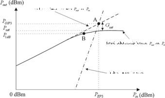
170 |
5 Critical Techniques of Quantitative System-Level EMC Design |
Fig. 5.45 Input/output transfer characteristics of a nonlinear amplifier
The 1 dB gain compression point is defined as the point where the difference between the amplifier linear gain and the actual nonlinear gain is 1 dB. It is used to measure the power capacity of the amplifier and indicates amplifier deviating constant. In the mixer, P1dB is the output power corresponding to the frequency when the functional relationship between the intermediate frequency (IF) signal and the RF input signal starts to deviate from the linear characteristic.
The third-order intercept (TOI) point is the intersection of the linear power extension line of the third-order intermodulation product and the linear power extension line of the first-order product. They correspond to the input intercept point and the output intercept point, respectively. The TOI point describes the degree of the thirdorder intermodulation distortion of the nonlinear amplifier. The further the TOI point is from the 1 dB compression point, the smaller the amplitude of the third-order intermodulation component.
The saturation point is the output power point at which the amplifier’s maximum output power reaches saturation. At this power value, the linearity of the amplifier is poor, but the efficiency is high.
The difference between the amplifier gain and the ideal linear gain is defined as the saturation point gain compression.
(1) Nonlinear behavioral modeling method
In general, the amplifier model has three types, namely the physical model for circuit simulation (device model), the behavioral model for system-level simulation, and the behavioral model based on the partial physical model (the gray box model). The amplifier model built based on equivalent circuit and device is more suitable for circuit-level simulations and can provide accurate simulation results. However, the system will be too complex, or the implementing cost will be too high due to the usage of device-level or transistor-level models. The behavioral model only depends on the input and output test data of the amplifier, such that the internal components
5.3 EMC Modeling Methodology |
171 |
of the amplifier are not required for modeling. Using nonlinear mathematical expressions can also simulate the nonlinear characteristics and memory effect of the actual amplifier, which is very suitable for system-level EMC simulation.
The nonlinear behavioral model of an amplifier is usually a nonlinear expression. A behavioral model describing the nonlinear characteristics and memory effect can be obtained by solving the coefficients of the mathematical expression using the input and output data. This behavioral model includes memoryless nonlinear behavioral models and memory nonlinear behavioral models. For narrowband systems, it is generally not necessary to consider the memory effect of the amplifier. However, in the case of a wideband signal input, the amplifier has a nonnegligible memory effect due to the existence of the bias network and the matching network in the amplifying circuit. The following section discusses the memoryless behavioral model and the memory nonlinear behavioral model of the amplifier. We also provide the applicable situations and performance characteristics of various different models.
(1)Memoryless behavioral model. For an amplifier, the memory effect is negligible when the input is a narrowband signal. The memoryless behavioral model can be represented by two algebraic functions of the instantaneous envelope amplitude, which describe the real and imaginary parts or the magnitude and phase of the output envelope component. Let the amplifier input signal be
x(t) A(t)e jφ(t) |
(5.140) |
|
The common memoryless Taylor polynomial is |
|
|
y(t) |
∞ |
|
an xn (t) |
(5.141) |
|
|
n 1 |
|
where an is a constant.
When considering the complex coefficients and ignoring even orders, the model is in the form
y(t) |
N |
|
a2n−1|x(t)|2(n−1) x(t) |
(5.142) |
n 1
where N is the order of the polynomial.
The advantage of the Taylor series behavioral model is that the relative magnitude of each order distortion is reflected by the coefficient. The model is suitable for systems with smaller nonlinear distortion order and memoryless.
Another memoryless behavioral model is the Saleh function polynomial model [47]. Two equations are used to describe the AM–AM and AM–PM characteristics of the system, respectively
172 |
5 Critical Techniques of Quantitative System-Level EMC Design |
|||
|
Ay [ A(t)] |
αA A(t) |
(5.143) |
|
|
|
|
||
|
1 + βA[ A(t)]2 |
|||
|
φy [ A(t)] |
αφ A(t)2 |
|
(5.144) |
|
1 + βφ [ A(t)]2 |
|||
where αA, βA, αφ , and βφ are the measured fitting parameters for the AM–AM characteristics Ay [ A(t)] and AM–PM characteristics φy [ A(t)] of the amplifier. The Saleh model is suitable for memoryless quasi-linear systems with weak nonlinearity.
(2)Memory nonlinear behavioral model. The memory nonlinear model can be categorized into linear (static) memory effect behavioral model and nonlinear (dynamic) memory effect behavioral model based on the different memory effects. So far, the linear memory behavioral model of an amplifier mainly refers to the Wiener model and Hammerstein model.
The Wiener model consists of a linear filter followed by a nonlinear function model. The output is expressed as [48]
|
N |
M−1 |
n |
y(k) |
|
||
bn |
am x(k − m) |
(5.145) |
|
|
n 1 |
m 0 |
|
where y(k) and x(k) are the output and input of the model, respectively; M and N are the memory length and highest order of the polynomial, respectively.
The Hammerstein model is a cascade of nonlinear models without memory effects and linear time-varying modules [49], i.e.,
|
M |
N |
n |
y(k) |
|
||
bm |
an x(k − m) |
(5.146) |
|
|
m 0 |
n 1 |
|
Other models such as parallel Hammerstein models, parallel Wiener models, and Wiener–Hammerstein models are nonlinear memory effect behavioral models.
The memory polynomial model [50] consists of several delay taps and nonlinear static functions. This model describes the amplifier’s unbalanced and dynamic AM–AM and AM–PM characteristics. The amplifier behavioral model of discretetime complex baseband is
M−1 |
N |
|
y(k) |
a2n−1,m |x(k − m)|2(n−1) x(k − m) |
(5.147) |
m 0 n 1
In fact, the memory polynomial model and the Hammerstein are same models with different structures. The polynomial model is also a Volterra series model that takes only the diagonal Volterra kernel. It is suitable for weakly nonlinear systems with memory effects.
5.3 EMC Modeling Methodology |
173 |
The RBF neural network model is a behavioral model describing the nonlinear characteristics of amplifiers in recent years. In this model, some input and output data points are used as training samples to calculate the model parameters, such that the dynamic nonlinear behavior of the amplifier can be reproduced. Neural network model has a rather high accuracy, and the computational complexity is also high; consequently, the complexity for modeling and simulating the EMC of the neural network model as a sub-module in the system increases. This book will not elaborate on the neural network model.
Volterra model is a generalization of the Taylor series model. Theoretically, the Volterra series can approximate a nonlinear continuous function with arbitrary precision. However, in fact, because the number of model parameters increases exponentially with the increase of model order and memory effect, the curse of dimensionality is likely to happen in function identification [51]. Therefore, Volterra model is usually only applicable to weak nonlinear time-invariant systems with attenuated memory. This book will give a specific description of the Volterra model and discuss how to simplify the model so that it can be applied to strong nonlinear systems.
(2) Simplification of Volterra series behavioral model
Volterra series is usually used to describe the behavioral characteristics of nonlinear circuits or systems. Compared with simulation calculations that include specific physical structures, Volterra series can greatly reduce the computational complexity and can be easily applied to system behavioral simulation. Modern wireless communication systems usually have the characteristics of high frequency, high speed, and wide frequency band. In many nonlinear modules such as the low-noise amplifiers and mixers, RF power amplifiers are the main source of nonlinear distortion. The distortion and out-of-band interference result from the nonlinear modules will be more serious because of the existence of memory effect, so it is necessary to accurately establish the behavioral model of the power amplifier with nonlinear characteristics of the memory effect. This is also an important topic in the research of RF power amplifier modeling. This book will use a typical RF power amplifier as an example to describe the nonlinear behavior of the RF power amplifiers using Volterra series.
(1) Volterra series model. The Volterra series was first proposed by the Italian mathematician Vito Volterra in 1889. It is a generalization of the convolution operation in linear system theory to the analysis of nonlinear systems.
Volterra series of continuous and discrete systems. In a continuous nonlinear time-invariant system, x(t) and y(t) denote the input and output signals of the system, respectively, and the Volterra series expression is
y(t) |
∞ |
|
yn [x(t)] |
(5.148) |
|
|
n 0 |
|
where yn [x(t)] is the n-th order component of the system response. The expression is
174 |
|
5 Critical Techniques of Quantitative System-Level EMC Design |
∞ |
∞ |
hn (τ1, τ2, · · · , τn ) x(t − τ1)x(t − τ2) · · · x(t − τn )dτ1dτ2 · · · dτn (5.149) |
yn [x(t)] |
· · · |
|
−∞ |
−∞ |
|
where hn (τ1, τ2, · · · , τn ) is the n-th order Volterra kernel.
When all of the Volterra kernels higher than second order are zero, the nonlinear system degenerates into a linear system. In addition, the Volterra kernel function is symmetric [52]. For example, the third-order kernel satisfies: h3(τ1, τ2, τ3) h3(τ2, τ1, τ3) · · · h3(τ3, τ2, τ1).
In general simulation process, we process the digital signal after signal sampling. The discrete form of Volterra series is
∞ ∞ |
∞ |
n |
|
y(k) |
· · · |
hn (i1, i2, · · · , in ) x(k − i j ) |
(5.150) |
n 1 i1 0 |
in 0 |
j 1 |
|
where x(k) and y(k) are the input and output signals, respectively; hn (i1, i2, · · · , in ) is the n-th order Volterra kernel.
In practice, sufficient accuracy can be obtained using a finite number of orders and a finite memory length, and the Volterra series is truncated to the sum of the finite terms. In the communication system, the input and the output are generally modulated signals. Assume the input signal of the RF power amplifier is x(t) Re[x˜ (t) · e jω0 t ] and the output signal is y(t) Re[y˜(t)·e jω0 t ], where ω0 is the carrier angle frequency, and x˜ (t) and y˜(t) are the complex envelope of the input and the output signals, respectively. The Volterra model of discrete-time complex baseband is
y(k) |
M−1 h |
1 |
(i) |
x(k |
− |
i) + M−1 M−1 M−1 h |
3 |
(i |
, i |
, i |
) |
|
x(k |
− |
i |
)x(k |
− |
i |
)x (k |
− |
i |
) |
|
|
|
|
|
||||||||||||||||
˜ |
|
˜ |
|
× ˜ |
|
|
|
|
˜ |
1 |
|
2 |
3 |
|
× ˜ |
|
|
1 |
˜ |
|
|
2 |
˜ |
|
|
3 |
|
|
|
|
|
|
|||||||||||
|
i 0 |
|
|
|
|
|
i1 0 i2 i1 i3 0 |
|
|
|
|
|
|
|
|
|
|
|
|
|
|
|
|
|
|
|
|
|
|
|
|
|
|
|
|
|
|
|
|
|
|||
|
+ M−1 M−1 M−1 M−1 M−1 h |
(i |
, i |
, i |
, i |
, i |
) |
|
x(k |
− |
i |
)x(k |
− |
i |
)x(k |
− |
i |
)x (k |
− |
i |
)x (k |
− |
i |
) |
|||||||||||||||||||
|
|
|
|
|
|
|
˜ 5 |
1 |
2 |
3 |
|
4 |
5 |
|
× ˜ |
|
|
1 |
|
˜ |
|
2 |
|
˜ |
|
3 |
˜ |
|
|
4 |
˜ |
5 |
|
||||||||||
|
i1 0 i2 i1 i3 i2 i4 0 i5 i4 |
|
|
|
|
|
|
|
|
|
|
|
|
|
|
|
|
|
|
|
|
|
|
|
|
|
|
|
|
|
|
|
|
(5.151) |
|||||||||
|
+ · · · |
|
|
|
|
|
|
|
|
|
|
|
|
|
|
|
|
|
|
|
|
|
|
|
|
|
|
|
|
|
|
|
|
|
|
|
|
|
|||||
|
h |
, i2, · · · , in ) is the n-th order complex Volterra kernel of the system; M |
|||||||||||||||||||||||||||||||||||||||||
where ˜ n (i1 |
|||||||||||||||||||||||||||||||||||||||||||
|
|
|
|
|
|
|
|
· |
) |
|
|
|
|
|
|
|
|
|
|
|
|
|
|
|
|
|
|
|
|
|
|
|
|
|
|
|
|
|
|
˜ |
|
|
|
is the length of the memory; ( |
is the complex conjugate of the signal; x(k) and |
||||||||||||||||||||||||||||||||||||||||||
y˜(k) are the input and the output complex envelope discrete signals, respectively. The symmetry of the kernel has been considered in Eq. (5.151). At the same time, using the band-limited modulation characteristic of the communication system, even-order terms are removed, and a limited Volterra series model with the order N and memory length M is truncated to use in the analysis.
Model parameter identification. The Volterra series model parameter identification is a process to find the Volterra kernel using the input and the output data. Assuming the sampling process starts from time k and a set of sampling data of length L is obtained, the input and the output matrixes of the system are
5.3 EMC Modeling Methodology |
|
|
|
|
|
|
|
|
|
|
|
|
|
|
|
|
|
|
|
|
|
|
|
|
175 |
||||||||||||||||||
|
|
|
|
|
|
|
|
|
|
|
X [X(k), X(k + 1), · · · , X(k + L − 1)]T |
|
|
|
|
|
|
|
(5.152) |
||||||||||||||||||||||||
|
|
|
|
|
|
|
|
|
|
|
|
Y [y˜(k), y˜(k + 1), · · · , y˜(k + L − 1)]T |
|
|
|
|
|
|
|
(5.153) |
|||||||||||||||||||||||
where |
|
|
|
|
|
|
|
|
|
|
|
|
|
|
|
|
|
|
|
|
|
|
|
|
|
|
|
|
|
|
|
|
|
|
|
|
|
|
|
|
|
|
|
X(k) |
|
[x(k), |
· · · |
, x(k |
− |
M + 1), |
x(k) |
2 x(k), x2(k)x (k |
− |
1), |
· · · |
, |
|
(5.154) |
|||||||||||||||||||||||||||||
|
|
|
˜ |
|
|
|
|
˜ |
|
|
|
|
|
| |
˜ |
|
| |
˜ |
|
˜ |
|
|
˜ |
|
|
|
|
|
|||||||||||||||
|
|
|x˜ (k)|N −1 x˜ (k), · · · , |x˜ (k − M + 1)|N −1 x˜ (k − M + 1)] |
|
|
|
|
|
|
|
||||||||||||||||||||||||||||||||||
The kernel vector of the system is defined as |
|
|
|
|
|
|
|
|
|
|
|
|
|
|
|
|
|||||||||||||||||||||||||||
H |
˜ 1 |
(0), |
· · · |
|
|
˜ |
1 |
(M |
− |
|
|
˜ |
3 |
|
|
˜ |
3 |
(0, 0, 1), |
· · · |
˜ |
3 |
(M |
− |
1, |
M |
− |
1, M |
− |
1), |
· · · |
, |
||||||||||||
|
[h |
|
|
, h |
|
|
1), h |
|
(0, 0, 0), h |
|
, h |
|
|
|
|
|
|
|
|||||||||||||||||||||||||
|
|
h |
(0 |
, |
· · · |
, |
0 |
, |
0) |
, h |
|
(0, |
· · · |
, 0, 1), |
· · · |
, h |
(M |
− |
1, |
· · · |
, M |
− |
1)]T |
|
|
|
|
|
|
|
(5.155) |
||||||||||||
|
|
˜ N |
|
|
|
˜ N |
|
|
|
|
|
˜ N |
|
|
|
|
|
|
|
|
|
|
|
|
|
|
|||||||||||||||||
The Volterra model in Eq. (5.151) can be written as |
|
|
|
|
|
|
|
|
|
|
|
|
|||||||||||||||||||||||||||||||
|
|
|
|
|
|
|
|
|
|
|
|
|
|
|
|
|
|
|
|
|
Y X H |
|
|
|
|
|
|
|
|
|
|
|
|
|
|
|
(5.156) |
||||||
The solution of the parameters in Eq. (5.156) is an estimation problem. The collected data is far more than the number of parameters to be estimated. We can use the least square method to solve this pure overdetermined problem. The estimated
ˆ
kernel vector H is [53]
ˆ |
|
(X |
X)−1 X Y |
(5.157) |
H |
|
However, when the order and memory length of the nonlinear system increase, the number of the Volterra kernel to be identified grows exponentially, and the elements in the matrix X X are easily correlated. That is, the matrix appears ill-conditioned so that the singular values may appear during the solution. When the number of the Volterra kernels to be identified is larger than the number of the mutually unrelated elements, the solution process becomes a pure underdetermined problem (the least
ˆ
L2 norm problem), and the estimated kernel vector is H [53]:
ˆ |
|
X |
(X X )−1Y |
(5.158) |
H |
|
After Volterra behavioral model is identified, the model needs to be verified. Many system performance indicators can be used to evaluate the accuracy of the model, such as the bit error rate (BER) and the adjacent channel power ratio. The normalized mean square error (NMSE) [54] is used here as
|
P |
2 |
|
|
y˜s − y˜smod |
|
|
N M S E 10 log |
s 1 |
|
(5.159) |
S |
|
|y˜s |2
s 1
176 |
5 Critical Techniques of Quantitative System-Level EMC Design |
where P is the number of sampling points; y˜smod is the output complex envelope of the model; y˜s is the simulation output complex envelope.
The smaller the NMSE, the higher the accuracy of the model is.
(2) Method for Volterra behavioral model simplification. Theoretically, the Volterra series can approximate the nonlinear continuous function with arbitrary precision. However, the number of identification parameters exponentially increases with the increase of model order and memory length, which easily leads to the curse of dimensionality in function identification. Although the number of parameters in the calculation of the power amplifier model can be reduced using the symmetry of the Volterra kernel and the band-limited characteristics of the communication system, the computational cost of the parameter identification is still large. Therefore, the Volterra series is usually used to handle weak nonlinear systems. The simplification method is to set the identification kernel to zero one by one and then estimate the variation of the model error, leaving only the kernels that have a large impact on the model. This method is complicated and time consuming. In order to reduce the complexity of the Volterra model, many special models have emerged, such as the Wiener model and the Hammerstein model. Both models are adapted to power amplifiers with linear memory effects, but the extraction of model parameters is still difficult [55]. The fast calculation of parallel behavioral model can effectively improve the data processing speed and reduce the calculation time, but the problem of reducing the number of model parameters remains [56]. The memory polynomial model only takes into account the diagonal Volterra kernel. When the nondiagonal Volterra kernel contributes more to the output of the Volterra model than the diagonal Volterra kernel, the accuracy of the memory polynomial model decreases.
In fact, in most RF power amplifiers, the memory effect becomes weaker over time. Additionally, the higher the order of the input components with memory effects, the smaller the effect they have on the output. In order to simplify the Volterra series model, two Volterra kernel parameter control factors are introduced with fixed order and memory length: One is an adjacent diagonal kernel control factor to remove the long memory delay component that has less influence on the output from input signal vector X in Eq. (5.152); the other is a dynamic deviation order control factor that removes the high-order components with memory from the input signal vector X in Eq. (5.152) and keeps the parameters that have a large impact on the output in the Volterra series model. Therefore, the parameters of the model can be greatly reduced under the premise of retaining the accuracy.
Adjacent diagonal kernel control factor: Only the diagonal Volterra kernel is
retained in the memory polynomial model, i.e., when i1 i2 · · · in , |
|||||||||||
˜ n |
(i |
1 |
, i |
2 |
, |
· · · |
, i |
n |
) |
|
0. In the case where the nondiagonal Volterra kernel’s con- |
h |
|
|
|
|
|
||||||
tribution to the output cannot be ignored, a looser restriction condition is needed. The adjacent diagonal Volterra kernel control factor S is introduced to retain the kernels near the diagonal Volterra kernel [52]. Taking the n-th order kernel as an example, by setting the integer value for S (0 ≤ S ≤ M − 1) to lose the constraint condition ( i p − iq ≤ S), we can gradually retain more kernels near the diagonal kernel: If max i p − iq
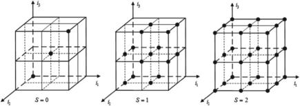
5.3 EMC Modeling Methodology |
177 |
Fig. 5.46 Quantity variation of the third-order Volterra kernel with the control factor S
kept. Figure 5.46 uses the third-order term (i.e., memory length M 3) as an example to illustrate the relationship between the control factor and the parameters to be
˜
identified. The origin of the coordinates is the Volterra kernel h3(0, 0, 0), and i1, i2, and i3 on the axes are all integers. For simplicity, we do not consider the symmetry of the Volterra kernel. It can be seen that: When S 0, Eq. (5.151) becomes the memory polynomial model; when S gradually increases, the identification parameter increases; when S M − 1, a complete Volterra series model can be achieved.
Dynamic deviation order control factor: When the order of the input signal with the memory in the power amplifier increases, its influence on the output will gradually reduce. The distortion of most power amplifiers is mainly caused by the memoryless nonlinearity and low-order memory nonlinearity. The previously discussed Taylor series model is actually a special form of the Volterra series, in which only the
h |
(i |
1 |
, i |
2 |
, |
· · · |
, i |
n |
) |
|
memoryless input is retained, i.e., when i1 i2 · · · in 0, ˜ n |
|
|
|
|
|
0. Another control factor R is introduced here to control the order of the memory input component of the input vector X in Eq. (5.152), which is called the dynamic deviation order control factor. R can also be interpreted as the maximum number of the nonzero elements in the set {i1, i2, · · · , in }, and 0 ≤ R ≤ N . For example, for the n-th order term, when R 1, there can only be one input component with memory, i.e., x˜ n−1(k)x˜ (k − i). Now taking the third-order term (i.e., memory length M 3) in Fig. 5.47 as an example, we will explain the relationship between the control factor and the parameters to be identified. The origin of the coordinates is
˜
the Volterra kernel h3(0, 0, 0), and i1, i2, i3 are rounded on the axis. It can be seen that: When R 0, Eq. (5.151) becomes a memoryless Taylor series model; when R gradually increases, the number of the identification parameters increases; when R N , the complete Volterra series model can be achieved.
Under the control of S or R, the number of Volterra kernel increases almost linearly with the increase of order and memory length.
However, both S and R are integers and have their own value range: 0 ≤ S ≤ M−1 and 0 ≤ R ≤ N . When the memory length M is large and order N is small, the value of S is large and the parameter changes can be controlled easily, but the value of R is small which results in fast parameter growth. Therefore, S is preferred as the control
178 |
5 Critical Techniques of Quantitative System-Level EMC Design |
Fig. 5.47 Quantity variation of the third-order Volterra kernel with the control factor R
factor. When the memory length M is small and order N is large, R is preferred as the control factor. When the memory length M and the order N are equal, the combination of the two factors shall be used.
In the actual power amplifier behavioral modeling process, combining the two control factors S and R, there will be four variables to control the model accuracy, which are the order N , memory length M, and the control factors S and R. Because the Volterra kernels generated using different S and R will partially overlap, here we use “or” to preserve the corresponding Volterra kernel parameters to be identified. By gradually increasing S and R, the number of parameters to be identified is controlled, such that the memory nonlinearity of the power amplifier can be described using less Volterra kernel.
(3) Verification of power amplifier behavioral model. In order to verify the simplified method of the power amplifier behavioral model, a 10 W power amplifier has been designed using the MRF6S21140H from Freescale. A commercial circuit software was used for simulation and raw data collection. When extracting parameters, in order to avoid the ill-conditioned matrix, and to fully reflect the nonlinearity of the power amplifier, Gaussian white noise signal is usually used as the input signal [54]. In
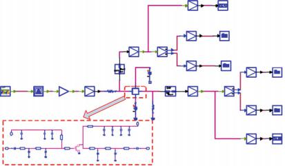
5.3 |
EMC Modeling Methodology |
|
|
|
|
179 |
||
|
|
|
|
|
|
Data Type Converter |
Spectrum Analyzer |
|
|
|
|
|
|
|
Data Type Converter |
Realtime Data Storage |
|
|
|
|
Data Type Converter |
Signal Converter |
|
|
||
|
|
|
CollectorSignal |
|
Source |
Data Type Converter |
Realtime Data Storage |
|
|
|
|
|
|
Data Type Converter |
Realtime Data Storage |
||
|
|
|
|
|
|
|
||
Source |
Filter |
Amplifier Data Type Converter |
Resistance |
Power Amplifier |
|
Data Type Converter |
Signal Converter |
|
|
|
|
|
|
|
|
|
|
|
|
|
|
|
|
Signal Collector |
|
Realtime Data Storage |
|
|
|
|
Source |
Resistance |
Data Type Converter |
||
|
|
|
|
|
|
|
||
|
|
|
|
|
|
|
Data Type Converter |
Spectrum Analyzer |
Fig. 5.48 Simulation of underlying circuit model with power amplifier
fact, the Gaussian white noise method is difficult in both simulation and experimental measurements, and the power amplifier is not used to amplify the Gaussian white noise signal. A WCDMA signal with an input code rate of 3.84 Mb/s was used as the input stimulus for the power amplifier with carrier frequency of 2.14 GHz. Figure 5.48 shows the simulation model that includes the power amplifier’s underlying circuits. The matching and biasing circuits in the amplifier’s underlying circuit were the main source of memory effects. This book regards the output of the simulation results of the circuit model as experimental data. About 4,000 input and output data points have been used for model parameter identification and validity verification.
The power amplifier circuit model is replaced with a Volterra series, of which the order N is 5 and the memory length M is 5.
First, the value of the control factors S and R was changed individually to analyze the goodness of fit of the model. Figures 5.49 and 5.50 show the partial time-domain complex envelope output waveforms for different behavioral models corresponding to different values of S and R, respectively. For the sake of clarity, only the real output waveform when both S and R were at the maximum value of 2 was considered. As the value increased, the output waveform of the behavioral model got closer and closer to the original data waveform.
For the different values of control factors, the number of parameters to be identified and the corresponding NMSE values are shown in Table 5.9.
When the NMSE is required to be no higher than −40 dB, the relative error between the model output and the simulated acquisition signal cannot be higher than 0.01%. As can be seen from Table 5.9, the requirement will be met with S 2 (203 identification parameters) or R 3 (225 identification parameters).
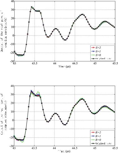
180 |
5 Critical Techniques of Quantitative System-Level EMC Design |
Fig. 5.49 Partial real part output waveforms of the time-domain complex envelope for behavioral models with different values of S
Fig. 5.50 Partial real part output waveforms of the time-domain complex envelope for behavioral models with different values of R
The memory effect of most power amplifiers gradually weakens as time goes by. At the same time, the influence from the input components with memory effect to the output gradually decreases as the order increases. Therefore, two control factors with large contribution to the output can be used to retain the input components, such that the number of parameters to be identified is further reduced. According to the data in Table 5.9, let S 1, R 2, and all Volterra kernels satisfying S 1 or R 2 are listed as parameters to be identified. The total number of identification parameters is 140 after calculation, and the corresponding NMSE is −40.2 dB. Figure 5.51 is the partial time-domain complex envelope waveform output from the power amplifier.
5.3 EMC Modeling Methodology |
181 |
Table 5.9 Number of parameters to be identified and the corresponding NMSE under different control factor values
|
|
|
|
|
Control factor |
The number of parameters to be |
NMSE |
||
|
|
identified |
(dB) |
|
|
|
|
|
|
S |
0 |
15 |
−37.2 |
|
|
1 |
71 |
−39.0 |
|
|
2 |
203 |
−40.2 |
|
|
3 |
407 |
−41.4 |
|
|
4 |
605 |
−42.2 |
|
R |
0 |
3 |
−30.3 |
|
|
1 |
23 |
−37.5 |
|
|
2 |
85 |
−39.5 |
|
|
3 |
225 |
−40.8 |
|
|
4 |
405 |
−41.7 |
|
|
5 |
605 |
−42.2 |
|
When S 1 and R 2, the output signal obtained from the simplification of the behavioral model can fit the actual output waveform well. In this case, the use of two control factors can better simplify the Volterra series model. The actual parameters to be identified are reduced from 605 to 140. Most of the extraneous parameters are eliminated, which greatly reduces the complexity of the solution matrix. Although the memoryless Taylor series model has a relatively small number of parameters, the deviation from the test data curve is still large (this is because the Taylor series model does not contain the term describing the memory effect), which can be seen from the results of the real part. It can also be seen that the power amplifier circuit has obvious memory characteristics, such that some memory items need to be reserved.
The signal output spectrum is further discussed based on the solved model. The behavioral model of the mathematical expression can be easily embedded in commercial circuit simulation software to build the digital circuit behavioral model containing the behavioral model of power amplifier, as shown in Fig. 5.52. Compared with Fig. 5.51, we suggest that time-domain simulator (envelope simulator) be removed from the model to reduce the transient time-domain calculations for the analog circuits.
Figure 5.53 shows the output spectrum of the input signal after passing through the power amplifier circuit. From the figure, we see that the output of the simplified Volterra model is basically the same as the output spectrum of the original circuit model and the out-of-band signal spectrum is exactly what is needed for the analysis of the abnormal EMC signals; since the memoryless Taylor model does not consider the memory effect, the out-of-band output spectrum power value is significantly reduced and does not accurately describe the out-of-band power spectrum.
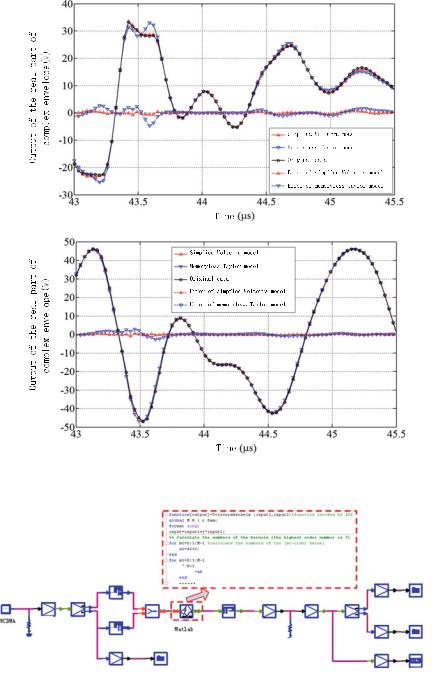
182 |
5 Critical Techniques of Quantitative System-Level EMC Design |
(a)
(b)
Fig. 5.51 Partial time-domain complex envelope output waveform for simplified behavioral model, a real part and b imaginary part
|
|
|
|
|
Data Type Converter |
Realtime Data |
|
|
|
Pack Module |
|
|
Storage |
||
Data Type Converter Signal Converter |
Bus merge |
Unpack Module |
Data Type Converter |
Signal Converter |
|
||
|
|
|
|||||
|
Resistance |
Pack Module |
|
|
|
|
Realtime Data |
|
|
Data Type Converter |
Resistance |
Data Type Converter |
Storage |
||
Source |
|
|
|||||
|
|
|
|
||||
|
|
|
Module |
|
|
|
|
|
|
|
|
|
|
|
|
|
|
Data Type Converter |
Realtime Data Storage |
|
Data Type Converter |
|
|
|
|
|
|
|
|
Spectrum Analyzer |
|
Fig. 5.52 Simulation of behavioral model including power amplifier