

5.3 EMC Modeling Methodology |
183 |
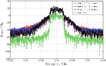
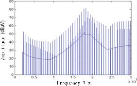
Fig. 5.53 Output spectrum of power amplifier behavioral model
5.3.3 EMC Modeling Method Based on Gray System Theory
Equipment’s EMC analysis model is the basis for EMC behavioral modeling. It is often required to specify the external electrical characteristics of the equipment and detailed design parameters for the EMC analysis model. However, in many applications, the electrical design parameters of the equipment are difficult to obtain, and even the key parameters including power and operating frequency cannot be accurately obtained. It also happens that the EMC behavioral model cannot be established due to the complex structure of the equipment. In order to obtain the main parameters of the equipment in the system-level EMC analysis, we propose a method which extracts the EMC characteristics of the equipment, such as the harmonic interference characteristics and the noise spectrum of the power supply through testing, generalize regular expressions for use in design, and further build EMC analysis model of the equipment/module under the condition of incomplete parameter information. This method is called the EMC modeling based on gray system theory method.
The incomplete information of the electronic system is categorized into four types: incomplete design information, incomplete structure information, incomplete boundary information, and incomplete system operation behavior information (response characteristics).
A system with incomplete information is called a gray system, where “gray” means “incomplete information.” In different scenarios and from different perspectives, the meaning of “gray” can also be extended. A gray system can be an intrinsic gray system or an extrinsic gray system. The basic characteristics of the intrinsic gray system are: There is no physical prototype, and there is no information to establish a definite relationship. The basic characteristics of the system are multiple parts that depend on each other, restrict each other, and are combined in a certain order. The intrinsic gray system has one or more kinds of functions. An extrinsic gray
184 |
5 Critical Techniques of Quantitative System-Level EMC Design |
system refers to a physical system whose information is temporarily unknown or not yet obtained. The research object of the gray system theory is the uncertainty system with “insufficient information.” The system has “part of information known and part of information unknown.” With this theory, the real world is described and understood through generation and developing of the “partial” known information. According to the gray system classification, the gray system modeling method also comes in categories: One is the hybrid method, which uses the deductive method for the white part with known information and the inductive method for the black part with unknown information. This method is applicable to extrinsic gray system; the other is gray system modeling method applied to intrinsic gray system.
The gray system modeling method reveals the internal movement law by processing gray information. It uses the system information to quantify the abstract concept, build model for the quantified concept, and finally optimize the model. It not only tries to isomorphize the system model using output information, but also attaches great importance to correlation analysis, so as to make full use of the system information and transform the disordered data into an ordered sequence suitable for modeling of differential equations. The gray system modeling method adopts gray number processing represented by interval and interval operations, which is a simple and practical method.
The idea for gray modeling: Through gray generation or sequence operators, the randomness is weakened and the potential laws can be discovered; through the interchange of gray difference equations and gray differential equations, continuous dynamics differential equations can be constructed using discrete data sequences.
The basic ideas of gray system modeling are: (1) qualitative analysis, quantitative modeling, and close combination of qualitative and quantitative analysis; (2) clarification of system factors, relationship between factors, and the relationship between the factors and the system (the relationship between factors and the relationship between the factors and the system are not absolute); (3) understanding the basic performance of the system through modeling; (4) system diagnosis through the modeling to reveal potential problems; (5) obtaining as much information as possible from the model, especially the changing information; the commonly used data for building models includes scientific experimental data, empirical data, and production data; the sequence generation data is the basis for establishing a gray model; (6) constructing gray differential equation for the data which might follows implicit rules;
(7) the model accuracy is set by gray numbers or gray sequences; (8) the accuracy of the model can be improved by different generation methods of gray data or gray sequence, data selection, sequence adjustment and correction, gray function form, and supplementation methods for different levels of residual gray model.
The gray system theory uses three methods to test and verify the accuracy of the model: residue size test, which is the point-by-point test of the error between the model value and the actual value; correlation test, which is a test by examining similarity between the model value curve and the modeling sequence curve; andposterior difference test, which tests the statistical characteristics of the residual distribution.
5.3 EMC Modeling Methodology |
185 |
(a) |
(b) |
2MHz |
1GHz |
10MHz |
200MHz |
(c)
30MHz |
200MHz |
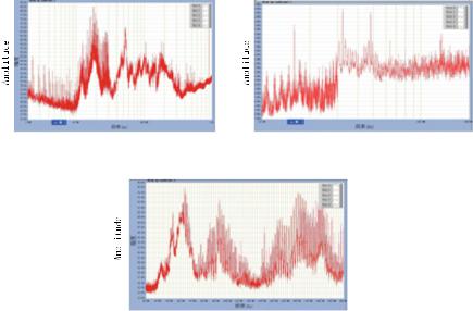
Fig. 5.54 Electromagnetic emission test data of three pieces of airborne equipment. a Equipment 1; b Equipment 2; and c Equipment 3
With the method of EMC modeling based on gray system theory, we can analyze the interference factors in the interference spectrum of the equipment, extract the harmonic interference and broadband interference information in the equipment, obtain the electromagnetic emission law of the equipment, and establish the EMC gray box model of the equipment based on the test data. The modeling accuracy is determined according to the least squares criterion.
One of the most important applications of the EMC modeling based on gray system theory is to investigate the potential interference sources and to design the corresponding EMC improvement schemes in the subsystem-level joint test and system-level precompliance test. Figure 5.54 is an example to illustrate the unique role of gray system method. The figure provides the electromagnetic emission test data for the three pieces of airborne equipment, respectively. As can be seen from Fig. 5.54, even for a single piece of onboard equipment, its electromagnetic emission data covers a wide range of frequencies which is usually hundreds of frequency octaves. When there are several pieces of such equipment in a system or a subsystem, the electromagnetic emission spectrum that they jointly produce will be more complicated. If a piece of equipment that works with these three pieces of equipment is susceptive, it is necessary to determine the cause of the susceptibility and design the interference suppression device.

186 |
|
|
|
|
5 Critical Techniques of Quantitative System-Level EMC Design |
|||||||||||||
|
|
|
|
|
|
|
|
|
|
|
|
|
|
|
|
|
|
|
|
|
|
|
|
|
|
|
|
|
|
|
|
|
|
|
|
|
|
|
|
|
|
|
|
|
|
|
|
|
|
|
|
|
|
|
|
|
|
|
|
|
|
|
|
|
|
|
|
|
|
|
|
|
|
|
|
|
|
|
|
|
|
|
|
|
|
|
|
|
|
|
|
|
|
|
|
|
|
|
|
|
|
|
|
|
|
|
|
|
|
|
|
|
|
|
|
|
|
|
|
|
|
|
|
|
|
|
|
|
|
|
|
|
|
|
|
|
|
|
|
|
|
|
|
|
|
|
|
|
|
|
|
|
|
|
|
|
|
|
|
|
|
|
|
|
|
|
|
|
|
|
|
|
|
|
|
|
|
|
|
|
|
|
|
|
|
|
|
|
|
|
|
|
|
|
|
|
|
|
|
|
|
|
|
|
|
|
|
|
|
|
|
|
|
|
|
|
|
|
|
|
|
|
|
|
|
|
|
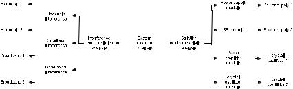
Fig. 5.55 Flowchart of the gray behavioral modeling and simulation of electronic system
In this situation, it is difficult to determine the main source of interference directly based on the electromagnetic emission test data. It is also difficult to design an effective interference suppression scheme (because the usual interference suppression program—filtering, shielding, etc.—is narrowband technology, while the frequency band of the emission spectrum as shown in Fig. 5.54 is very wide). For large systems (e.g., the system contains dozens of equipment), it is more difficult to identify the sources of interference and design effective suppression schemes.
The EMC modeling based on gray system theory method proposed in this book is very effective in solving this kind of problem. We will introduce the EMC modeling based on gray system theory method and provide examples of applications in the following paragraphs.
In general, electronic equipment includes units such as power supply, analog circuits, digital circuits, power amplifiers, and filtering. The communication system also includes nonlinear devices such as power amplifiers, mixers, and antenna matching networks. The external emission characteristics of the equipment are the combined emission characteristics of the various units above. In order to obtain the internal emission characteristics of the equipment from the external characteristics, it is necessary to test the emission characteristics of the equipment based on the internal potential interference module of the equipment. The test data is used to decompose and extract the external emission characteristics of each interference module to establish the behavioral model for different modules. Finally, we can build a behavioral model of the equipment based on the behavioral models of each module according to the equipment characteristics. The electronic system gray behavioral modeling simulation flow is shown in Fig. 5.55.
5.3 EMC Modeling Methodology |
187 |
From the perspective of EMC, the radiation interference from most systems can be categorized into harmonic interference and broadband interference. According to the gray behavioral modeling and simulation method and the electrical characteristics of the system, we can decompose the emission spectrum characteristics of the known system according to the different spectral distribution characteristics and use the test data to deduce the gray function of the spectral distribution of various characteristics to establish a gray behavioral model of external emission characteristics of the entire electronic system. In order to fully explain how to extract the gray function from the test data and establish a gray behavioral model of electronic system, we divide the modeling method into two steps: The first step is to establish a gray behavioral model for the single emission law of electronic systems; the second step is to study the gray behavioral model of the complex electronic systems with multiple emission characteristics.
1.Establish a simple gray behavioral model for single emission interference characteristics of the electronic system
For a simple emission interference system, its emission test data contains a single regular emission spectrum characteristic. According to the gray system theory, a gray function can be used to quantify the spectral distribution, and then a mathematical function can be used to establish a behavioral model under a single characteristic of a simple emission system. Assume that according to the preliminary judgment of the characteristics of the electronic system, the test data X {xi (k)(k 1, 2, . . . , m, i 1, 2, . . . , n) } is obtained, where m indicates the data length and n is the time of repeated test to avoid the influence of the environment on the test data. The test data can be abbreviated as X {xi (k) }. The method for establishing a gray behavioral model for a single emission law of an electronic system is as follows:
(1) Extract test data and construct a reference data sequence. In order to reduce the test error in the test data, data at the k-th point is used as the center to calculate the
1 |
n |
|
{x0(k) } |
arithmetic average x0(k) n |
i 1 xi (k), of the test data of the n group. X |
is used as the reference data sequence.
(2) Extract the gray sequence according to the maximum correlation. The gray correlation of the gray data sequence is defined as
r(x, x |
0 |
) |
|
ξ d(x, x0) |
(5.160) |
|
|x − x0|+ξ d(x, x0) |
||||||
|
|
|
where r(x, x0) is the gray correlation between x and x0. The larger the value of r(x, x0), the closer the correlation; d(x, x0) is the correlation distance between x and x0; ζ is the resolution coefficient and ξ (0, 1]. We take ξ 0.5.
ˆ |
n sequences can be substituted to calculate the gray correlation. The data sequence |
||
ˆ |
|
1, 2, . . . , m) with the greatest gray correlation with the reference |
|
X |
x(k)(k |
|
|
data sequence can be extracted, namely gray sequence.
(3) Create a gray function. According to the regularity trend of gray data series, we can assume the corresponding gray function form. For example, for a series
188 |
5 Critical Techniques of Quantitative System-Level EMC Design |
that approximates an exponential trend, it can be assumed that the data satisfies the exponential equation. We can then calculate and build a gray function
xˆ (0)(k) + axˆ (1)(k) b |
(5.161) |
where a, b are parameters.
Thus, the gray model of the exponential series is
dxˆ
+ axˆ b (5.162)
dt
For the common form of mathematics law, there are well-defined gray function forms and function parameter calculation methods, which generally meet the requirements of extracting the corresponding law functions and establish the gray model.
(4) Solve the parameters of the gray function. The gray function can be written as
|
|
|
|
Y φθ |
|
|
|
(5.163) |
|
where |
|
|
|
|
|
|
|
|
|
|
|
xˆ (0)(2) |
|
|
−xˆ (1)(2) 1 |
|
|
|
|
Y |
|
xˆ (0)(3) |
, φ |
|
−xˆ (1)(3) 1 |
, θ |
|
a |
|
. |
. |
. |
b |
||||||
|
. |
|
. |
. |
|
|
|||
|
|
. |
|
|
. |
. |
|
|
|
|
|
xˆ (0)(m) |
|
|
−xˆ (1)(m) 1 |
|
|
|
|
Then, the least square estimation parameter of the gray function is |
|||||||||
|
|
[a, b]T |
φT φ −1φT Y |
|
|
(5.164) |
|||
(5)Create a gray expression. Substitute each parameter into a gray function, and the gray function expression of the test data is
xˆ ( f ) (xˆ ( f0) − b/a)e−a |
f |
|
|
f0 |
+ a/b |
|
|
Ce− A f + B, f [ fmin, fmax] |
(5.165) |
||
where the independent variable f represents the frequency of the test data; A, B, and C are
A |
a |
, B a/b, C xˆ ( f0) − b/a |
(5.166) |
f0 |
This way, a large amount of data is simplified into a simple mathematical expression that facilitates modeling and simulation.
5.3 EMC Modeling Methodology |
189 |
(6)Create a gray behavioral model based on the expression. Substitute the gray expressions into the behavioral simulation system; thus, we can establish a gray behavioral model of a simple system with single law.
2.Establish a gray behavioral model of a complex emission system under multiple radiation conditions.
For complex electronic systems, there are many factors that affect the emission characteristics of the system. When electromagnetic interference analysis is performed, the original test data must include a variety of implicit laws. Various regular gray data sequences can be extracted from the original test data. According to the gray system theory, the regularity of one can be improved by transformation, and the influence of the other laws can be reduced. Thus, a regular gray sequence analysis formula can be obtained first, and a single characteristic behavioral model can be established. Then, we can identify the factors that make up the system and the correlation between the factors, and gradually obtain other regular gray sequences, so as to establish a complex system gray behavioral model containing multiple emission characteristics. The modeling method is as follows:
(1)Determine the gray characteristics of the system. As mentioned before, the type of externally emitted interference from the electronic system can be generally categorized into harmonics with periodic distribution of frequencies and broadband interference with continuous distribution; e.g., the electronic systems have different forms of power supply which have different emission characteristics. A common switching power supply exhibits harmonic characteristics externally. The AC power supply exhibits broadband characteristics externally. Different interference components have different frequency distributions, different amplitudes, and different influences. At the same time, different functional modules within the system will also show a variety of distribution forms; for example, the crystal oscillator and the switching power supply will exhibit harmonic interference characteristics, but the general harmonic frequency of the crystal is higher. Therefore, according to the existing EMC knowledge, we may analyze the possible functional modules and interference components in the system from the external output spectrum test data, infer the internal characteristics of the system from the external test data, and establish a behavioral simulation model.
Figure 5.56 shows an example of the decomposition of interference emitted by an electronic system. The gray function and gray model of each module are clearly defined according to the type of spectrum to establish a gray behavioral model of the
entire electronic system. Suppose the system has g number of gray modules, gray characteristics can be described using the g gray model functions fi(i 1, 2, . . . , g) such that the number and type of models can be evaluated.
(2)Determine the functional form of each gray characteristic. In the system behavioral model, the exact function expressions of each gray module are given according to the harmonic model and the broadband model, and then the gray behavioral description function corresponding to each gray module is obtained. If the form of
190 |
|
|
|
|
|
|
|
5 Critical Techniques of Quantitative System-Level EMC Design |
||||||||||||||||
|
|
|
|
|
|
|
|
|
|
|
|
|
|
|
|
|
|
|
|
|
|
|
|
|
|
|
|
|
|
|
|
|
|
|
|
|
|
|
|
|
|
|
|
|
|
|
|
|
|
|
|
|
|
|
|
|
|
|
|
|
|
|
|
|
|
|
|
|
|
|
|
|
|
|
|
|
|
|
|
|
|
|
|
|
|
|
|
|
|
|
|
|
|
|
|
|
|
|
|
|
|
|
|
|
|
|
|
|
|
|
|
|
|
|
|
|
|
|
|
|
|
|
|
|
|
|
|
|
|
|
|
|
|
|
|
|
|
|
|
|
|
|
|
|
|
|
|
|
|
|
|
|
|
|
|
|
|
|
|
|
|
|
|
|
|
|
|
|
|
|
|
|
|
|
|
|
|
|
|
|
|
|
|
|
|
|
|
|
|
|
|
|
|
|
|
|
|
|
|
|
|
|
|
|
|
|
|
|
|
|
|
|
|
|
|
|
|
|
|
|
|
|
|
|
|
|
|
|
|
|
|
|
|
|
|
|
|
|
|
|
|
|
|
|
|
|
|
|
|
|
|
|
|
|
|
|
|
|
|
|
|
|
|
|
|
|
|
|
|
|
|
|
|
|
|
|
|
|
|
|
|
|
|
|
|
|
|
|
|
|
|
|
|
|
|
|
|
|
|
Fig. 5.56 Decomposition of the emission type of an electronic system
the module is relatively complex, we can use a combination of multiple piecewise functions to create the exact function of the behavioral model.
(3) Establish the gray behavioral model of each gray module according to the system emission characteristics. For the same gray module, the gray function has the same form, and the variable forms of the function should also be the same. Assuming that the i-th module has n functions and each function has g parameters, we can create a parameter matrix in the form of the same type of function in the module.
|
|
R1 |
|
ri11 |
ri12 · · · ri1g |
|
||
|
|
R2 |
|
|
||||
Ri |
|
|
ri21 |
ri22 · · · ri2g |
(5.167) |
|||
. |
. |
. |
. |
. |
||||
|
. |
. |
. |
. |
. |
|
||
|
|
. |
|
. |
. |
. |
. |
|
|
|
Rn |
|
rin1 rin2 · · · ring |
|
|||
(4) Calculate the error of each model and modify the models. Compare the gray sequence of each module with the output of the model, and ensure that the model’s error is less than 3 dB when the output data converges; otherwise, adjust the gray function form or raw data interval and recalculate until the model’s error is less than 3 dB. The error calculation formula is
e max xˆ (k) − x(k) , (k 1, 2, . . . , m) |
(5.168) |
(5) Establish a gray behavioral model of the entire complex electronic system. On the basis of the behavioral model of each module, according to the overall emission of the system and the cross-linking relationship between the modules, the gray behavioral model of the system is established. The inter-system EMC analysis focuses on the external emission characteristics of the system. Although the current distribution and transmission path within the system are not clear, a behavioral model in which the transmission output is consistent with the actual system can still be established on the simulation platform.
3. An example of gray behavioral modeling
5.3 EMC Modeling Methodology |
191 |
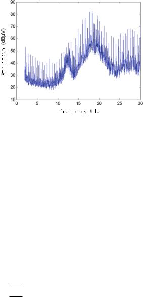
Fig. 5.57 Test spectrogram of an electronic system
We will use an example to describe the entire process of the gray behavioral modeling method of the system emission characteristics in detail. The tested external emission spectrum of an electronic system is shown in Fig. 5.57. The test spectrum is 2–30 MHz, and the frequency interval is 10 kHz.
Through the analysis of spectrum, there are multiple interference sources with different principles and functions in the system. It can be identified that the harmonic interference and broadband interference coexist. It can be initially determined that there are three interference sources in the system (two with harmonic characteristic and one with broadband characteristic), and the interference energy is mainly concentrated in the broadband interference. Assume that the original test sequence is X {x(k) }, and the broadband gray sequence XW {x(k) } (the subscript W denotes the broadband interference component) is extracted according to the principle of maximum correlation. The gray sequence of the first and second harmonics is X H 1 {xH 1(k) } and X H 2 {xH 2(k) }.
Assuming that both the harmonic component and the broadband component satisfy the exponential function, then the broadband component and the harmonic component can be represented by a set of exponential mathematical models
dxw1 + aw1 dt
dxw2 + aw2 dt
dxwg |
+ awg x |
|
dt |
||
|
x bw1 |
|
x bw2 |
(5.169) |
.. . . . .
bwg
where g is the number of exponential model in each interference component. The mathematical model of the broadband interference is
192 |
5 Critical Techniques of Quantitative System-Level EMC Design |
Fig. 5.58 Output of the gray system simulation model
xˆw1( f ) C1e− A1 f xˆw2( f ) C2e− A2 f xˆw3( f ) C3e− A3 f
+ B1, f1 [2M, 15M) |
(5.170) |
|
+ B2, f2 |
[15M, 22M) |
|
+ B3, f3 |
[22M, 30M] |
|
After the decomposition of the emission characteristics of each interference module in the system, gray sequence of each component is extracted. Then, we can calculate the function parameters of each interference component and define the function of analytical expression. The parameter transposed matrix for the broadband interference is
5.014 |
× |
10−5 |
1.11453 |
× |
10−4 |
5.98319 |
× |
10−4 |
|
|
|
|
|
||||||
4.5971 |
−0.1092 |
0.7430 |
(5.171) |
||||||
−4.187 |
0.3624 |
−0.0570 |
|
||||||
After getting the gray function of each interference component, the gray behavioral model of each module is established, and the behavioral simulation results of each module are compared with the actual characteristics to ensure that the EMC simulation output error is less than 3 dB. Figure 5.58 shows the gray system model simulation output of this electronic system. Based on the gray model of the above modules, the overall behavioral simulation model of the system is established, as shown in Fig. 5.59.
Due to the effective differentiation of each module, the EMC design method to reduce the external emission of the system is predicted using the behavioral simulation method. For different interference modules, the corresponding quantitative suppression requirements and improvement measures are clearly defined, which can effectively solve problems such as harmonic interference, broadband interference, and environmental noise interference. In practical applications, we can take specific measures: Add port filters for the two types of harmonic interference sources; add power filters that suppress broadband interference to the power supply.