Industrial Control (Students guide, 1999, v1.1 )

Experiment #2: Digital Input Signal Conditioning

Figure 2.11a and b: Retro-reflective Switch Pictorial and Schematic

Industrial Control Version 1.1 •Page 49

Experiment #2: Digital Input Signal Conditioning

Adjust the potentiometer to provide the proper reference voltage, which is halfway between the measurements.

Testing the output of the LM358 should result in a signal compatible with the BASIC Stamp. The output should be low with no object and high when the white object is placed in front of the emitter/detector pair. Measure these two output voltages of the LM358 and record the values in Table 2.3. If the output signal is compatible, apply it to the BASIC Stamp’s Pin 3. Detecting light reflected by an object is called retro-reflective detection.

Table 2.3: LM358 Values

This ability to yield a switching action based on light received lends itself to many industrial applications such as product counting, conveyor control, RPM sensing, and incremental encoding. The following exercise will demonstrate a counting operation. You will have to help, though, by using your imagination.

Let’s assume that bottles of milk are being transferred on a conveyor between the filling operation and the case packer. Cut a strip of white paper to represent a bottle of milk. Passing it in front of our switch represents a bottle going by on the conveyor. Only a slight modification of the previous program is necessary to test our new switch. If you have Program 2.5 loaded, simply modify the first button instruction by changing the input identifier from Pin 1 to 3. The modified line would look like this:

'Program 2.6 (modification to Program 2.5

'for the retroreflective switch input)

BUTTON 3,1,255,0,Wkspace1,1,Count_it

' Debounced edge trigger detection of optical switch

Programming Challenge #2: Milk Bottle Case Packer

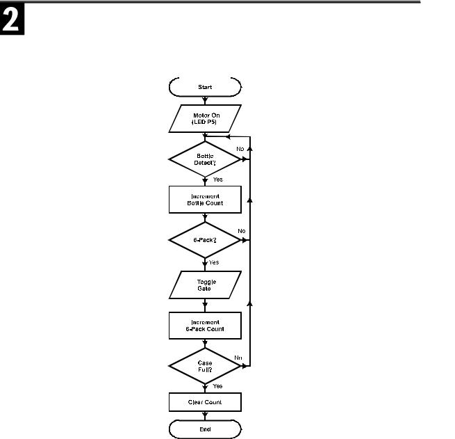
Refer back to Experiment #1 and consider the conveyor diverter scenario in Figure 1.2. We will assume that the controller is counting white milk bottles. Our retroreflective switch detecor could replace the “Detector1” switch in the original figure. The active high PB1 would toggle the conveyer motor ON and OFF. The LED on P4 can indicate that the motor is ON by lighting up. The LED on P4 is controlling the diverter gate. When high the gate is to the right and when low,the gate is to the left. Your challenge is to start the motor with PB1 and count bottles as they pass. Each sixth bottle, TOGGLE the diverter gate’s position as indicated

Page 50 •Industrial Control Version 1.1

Experiment #2: Digital Input Signal Conditioning

by the ON and OFF status of the LED on P4. After a case (4 six-packs) have been diverted t each side, turn off the motor. The process would start over by pressing the pushbutton again. Refer to Flowchart 2.12 to gain an understnding of the program flow.

Figure 2.12: Flowchart of Milk Bottle Challenge

Industrial Control Version 1.1 •Page 51

Experiment #2: Digital Input Signal Conditioning

Exercise #5: Tachometer Input

Monitoring and controlling shaft speed is important in many industrial applications. A tachometer measures the number of shaft rotations in a unit of time. The measure is usually expressed in revolutions per minute (RPM).

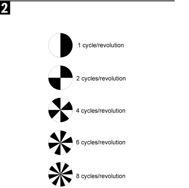
A retroreflective switch can open and close fast enough to count white and black marks printed on a motor’s shaft. Counting the number of closures in a known length of time provides enough information to calculate RPM. Figure 2.13 represents five possible encoder wheels that could be attached to the end of a motor shaft. If the optical switch is aimed at the rotating disk, it will pulse on-off with the alternating segments as they pass. The number of white (or black) segments represent the number of switch cycles per revolution of the shaft. The first encoder wheel has one white segment and one black segment. During each revolution, the white segment would be in front of our switch half the time, resulting in a logic high for half the rotation.

During the half rotation the black segment is in front of the disk, it absorbs the infrared light and with no reflected light, the switch will be low. One cycle of on-off occurs each revolution. The PBASIC2 instruction set provides a very useful command called COUNT that can be used to count the number of transitions at a digital input occuring over a duration of time. Its syntax is shown below.

PBASIC Command Quick Reference: COUNT

COUNT pin, period, variable

•Pin: (0-15) Input pin identifier.

•Period:(0-65535) Specifies the time in milliseconds during which to count.

•Variable: A variable in which the count will be stored.

The following exercise uses the count instruction, the optical switch, and the shaft encoder wheels to capture speed data.

Lets begin by cutting out the first encoder wheel. Fold a piece of cellophane tape onto the back of the encoder wheel to hold it on the shaft hub of the fan motor (a full-size set of encoder wheels may be pulled from Appendix B of this text). The fan is rated at 12 V. Its speed changes with varying voltages from 12 V down to approximately 3.5 V. This is the dropout voltage of the brushless motor control circuitry. Test your fan by directly connecting it across the Vdd (+5 volt supply) and then test it across the +Vin (unregulated) supply. Pin 20 of connector X1 provides access to the unregulated supply (Vin). You must observe the poalarity on brushless motors. The red lead is positive (+V) and the black lead is connected to Vss. The fan should be located so the encoder wheel is pointed at the emitter/detector pair.

Page 52 •Industrial Control Version 1.1

Experiment #2: Digital Input Signal Conditioning

Figure 2.13: Retro-reflective Encoder Wheels (cutouts are available in Appendix B)

Industrial Control Version 1.1 •Page 53

Experiment #2: Digital Input Signal Conditioning

The first encoder wheel has one white and one black segment on it. As it rotates, the opto-switch should cycle on-off once for each revolution. Enter the Tachometer Test Program 2.7 below.

'Program 2.7 Tachometer Test - with the StampPlot Interface

'Initialize plotting interface parameters.

'(Can also be set or changed on the interface)

As the fan spins, the cycling of the photo switch will be counted for 1000 milliseconds (one second). With the duration of the Counts routine being one second and one cycle occurring with each rotation, we get the cycles per second of fan rotation. Most often, the speed of a rotating shaft is described in terms of revolutions per minute (RPM). Multiplying the revolutions per second times 60 converts cycles per second to RPM.

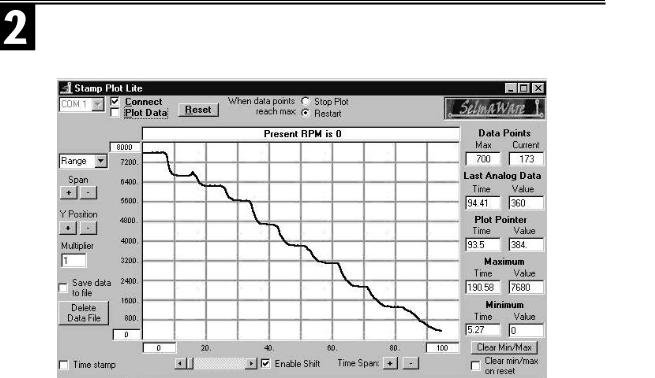
Run your program. The debug window will first appear with the serial information for configuration and display of the StampPlot Lite interface. Close the BASIC Stamp debug window and open StampPlot Lite. Check “Connect and Plot Data” and click on “Restart.” Press the Board of Education reset button and your interface should start plotting. Figure 2.14 shows a representative screen shot of the interface plotting RPM at various motor voltages.

Page 54 •Industrial Control Version 1.1

Experiment #2: Digital Input Signal Conditioning

Figure 2.14: RPM of the Brushless DC Fan at Varying Voltages

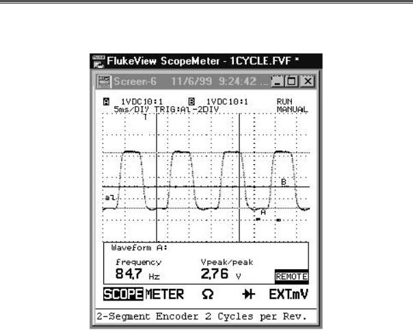
The spinning encoder wheel may result in a slightly different phototransistor peak output for “light” and “nolight” conditions. If your system is not reporting correctly, change the setpoint by adjusting the potentiometer to the new average value. If you have access to an oscilloscope, measure the peak-to-peak output of the phototransistor and your potentiometer setpoint being applied to the comparator. Placing the setpoint midway between the peak-to-peak DC voltage levels would allow for optimal performance. Notice the frequency and wave shape of the signal. An example of the oscilloscope reading is pictured in Figure 2.15. The 84.7 Hz equated to a debug readout of “Counts = 84 RPM = 5040.” The 84.7 Hz measured by the oscilloscope reflects an actual RPM of 84.7 x 60 = 5,082. Only 84 complete cycles fell within the one-second capture time of our routine.

Industrial Control Version 1.1 •Page 55

Experiment #2: Digital Input Signal Conditioning

Figure 2.15: Two-Segment Encoder Oscilloscope Trace

Record your tachometer readout when the maximum voltage is applied to the motor. You can use the Board of Education’s Vin (unregulated 9 V) for high speed, or the Vdd (regulated 5 V) for different speeds.

Counts = ___________ RPM = _____________

When testing your tachometer, notice the effects of slowing the motor with slight pressure from your finger. The counts will decrease by factors of one. In the Figure 2.13 example, it would decrease from 83 to 82 to 81, etc., and the resulting RPM readings drop by a factor of 60 (4980 to 4920 to 4860, etc.).

Page 56 •Industrial Control Version 1.1

Experiment #2: Digital Input Signal Conditioning

Because we are counting for one second and we get one cycle per revolution, the program can resolve RPM only to within an accuracy of 60. To get a more accurate assessment of RPM, you have a couple of choices: increase the time you count cycles, or increase the cycles per revolution.

Let’s try the first choice. Increase the count time in Program 2.7 from 1000 milliseconds to 2000 milliseconds. By doing so, you are now reading during a two-second window and RPM would equal {(Counts/2 seconds) x 60}. This simplifies to RPM = 30 * Count and the resolution is now to within 30 RPM. In program 2.7, change the line RPM = Counts * 60 from the scaling value of 60 to 30. Test your system.

Increasing the count duration time increases the accuracy of the RPM reading. Refer to Table 2.4.

Table 2.4: Given Encoder Frequency of 84.7 Hz

From the 1 cycle/second Encoder is an RPM of 5082

As you can see, to gain a resolution of one RPM, our count routine had to be one full minute (60,000) in duration. Unless you are very patient, this is unacceptable! In terms of programming, the BASIC Stamp is tied up with the COUNT routine for the total duration. During this time, the rest of the program is not being serviced. For this reason, long duration also is not good.

Another method of improving resolution is to increase the number of cycles per revolution. Cut out the second encoder wheel and tape it to your fan motor hub. This wheel has two white segments and will produce two count cycles per revolution. During a one-second-count duration, this encoder will produce twice as many pulses as the first encoder. The RPM calculation line of the code would be RPM = Counts x 60 / 2 for this encoder, or RPM = Counts x 30. Try it!

The third encoder wheel yields even more resolution by with four cycles per revolution. Tape this encoder to your motor’s hub and change the program’s RPM line to RPM = Counts * 15. You may have to vary the setpoint potentiometer as you switch from one encoder wheel to another.

Industrial Control Version 1.1 •Page 57

Experiment #2: Digital Input Signal Conditioning

If you use the six-cycle encoder, what value would you use to scale the Counts to RPM? Fill in your answer in Table 2.5.

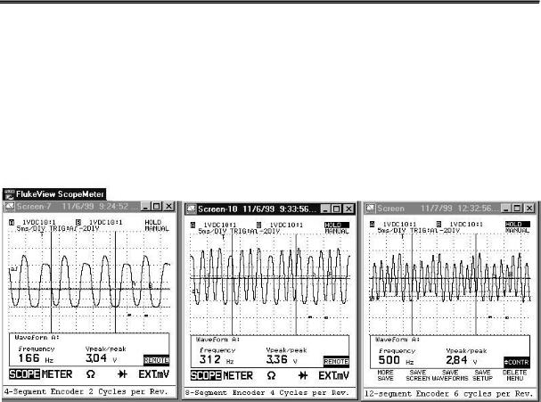
Figure 2.16 includes oscilloscope traces recorded from using the two-cycle, four-cycle, and six-cycle encoder wheels on a shaft rotating at 4,980 RPM. It is the focal properties of the emitter/detector pair that will limit the maximum number of segments on the encoder wheel. You may find it difficult to use the six-cycle encoder wheels without devising some sort of shielding and/or focusing of the light beam.

Figure 2.16: Two-cycle, Four-cycle, and Six-cycle Encoder Wheel Oscilloscope Traces

The accuracy required of a tachometer system is dependent on the application. Commercial shaft encoders are available with resolutions greater than 500 counts per revolution. Fill in the appropriate values in Table 2.5 for an encoder with a resolution of 360 counts per revolution.

Page 58 •Industrial Control Version 1.1