Industrial Control (Students guide, 1999, v1.1 )

Experiment #4: Continuous Process Control

Figure 4.5: Zero and Span Settings for Our Application

Industrial Control Version 1.1 •Page 109

Experiment #4: Continuous Process Control

With these settings, the ADC0831 is focused on a temperature range of 70 to 120 degrees. There can be an infinite number of possible temperature values within the .7 to 1.2-volt output range of the LM34. Only a few representative values are given. Since the 8-bit A/D converter has a resolution of 255, it can resolve this range of 50-degree temperatures to within .31 degrees. The conversion will be a binary number equal to [(Vin - .7) /.5] *255. Let’s try a value within the range. Let’s say the temperature is 98.6, which results in an LM34 output of .986 volts.

If Vin = .986, what would be the binary equivalent?

[(.986-.7)/.5] *255 = 145.86. The answer is truncated to the whole integer of 145. The binary word would be 1001 0010.

The binary conversion will be held and ready for transfer.

The SHIFTIN instruction is designed for synchronous communication between the BASIC Stamp and serial devices such as the ADC0831. The syntax of the instruction is SHIFTIN dpin, cpin, mode, [result\bits]. The parameters indicate:

•which pin data will arrive on (dpin),

•which pin is the clock (cpin),

•(mode) identifies which bit comes first, the least significant (LS) or most significant (MS), and on which edge of the clock it is released, rising (PRE) or falling (POST),

•and, what the word width is and where you want it stored [Datain\8].

For our system, we previously declared Pin 5 as dpin and Pin 4 as the clock (CLK) pin. The ADC0831 outputs the most significant bit first on the trailing edge of the clock. Therefore, MSPOST is the mode. And, finally, the 8- bit data will be held in a byte variable that we declared as Datain.

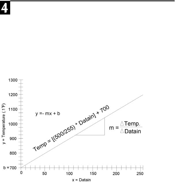
After the binary data is brought into the BASIC Stamp, it is available for our program to use. It would be most convenient to use if it were expressed in terms of the actual measurement units. For our application, that would be in degrees. The next subroutine, Calc_Temp, does just that. By knowing the zero and span transfer function of the conversion process, we use the standard y = mx + b formula. Where: y =Temperature, m = slope of the transfer function, and b is the offset. Temperature will be resolved and expressed in tenths of degrees.

Refer to the Calc_Temp formula: Temp = Tempspan/255 * Datain/10 + 700

Page 110 •Industrial Control Version 1.1

Experiment #4: Continuous Process Control

To increase the accuracy in resolving the slope (m), the Tempspan variable is scaled up by 10, to 5000 hundredth degrees. The slope is therefore, 5000/255 ~ 19 or .19 degrees per bit. Multiplying 19 times Datain tells you how far the measurement is into the span. This is in one one-hundredth of a degree at this point; therefore, divide by 10 to scale it back to tenths. Adding this to the Zero value of 700 (70 degrees) results in the actual temperature in tenths of a degree. Resolution is approximately .2 degrees over a range of inputs from 70.0 to 120.0 degrees.

The graph in Figure 4.6 plots the transfer function of the input A/D decimal equivalent input to temperature of the canister. Changing the span of coverage changes the slope of the transfer function. Changing the Zero value changes the y intercept.

Figure 4.6: Transfer Function

Industrial Control Version 1.1 •Page 111

Experiment #4: Continuous Process Control

An additional word of caution about the BASIC Stamp math operation:

•A formula will be executed from left to right unless bracketing is used to set precedence.

•At no point can any subtotal exceed 32,759 or -32,760.

•Also, all remainders will be truncated, not rounded up.

Challenge #1: Change the Zero and Span voltages and edit the program to match the new range.

1.Your system should be able to raise the temperature of the closed canister beyond the 120-degree limit set by Program 4.1. Change the Zero and Span potentiometers for coverage of a temperature range from 75 degrees to 200 degrees. This allows for a wider range of coverage, but what is the resolution of your system now? Be patient, and let your system stabilize. Record the maximum temperature of your system.

2.Set the Zero and Span of your system to focus on the very narrow range of one degree below your room temperature to four degrees above it. Set the Calc_Temp variables to display in hundredths of degrees. Track these changes by leaving the cap off of the canister and simply touching the sensor with your warm finger. As you see, the resolution is great, but the trade-off is a decreased range of operation.

Having the ability to control the span and reference of the ADC0831 allows you to focus on a range of analog input. This helps maximize the resolution and accuracy of your system. The following exercise will require the original range of 70 to 120 degrees. Return the Zero and Span potentiometers back to .7 and .5 volts, respectively.

Now, after all of that, we can get back to a study of control theory!

Page 112 •Industrial Control Version 1.1

Experiment #4: Continuous Process Control

Exercise #2: Open-Loop vs. Closed-Loop Control

Open-Loop Control

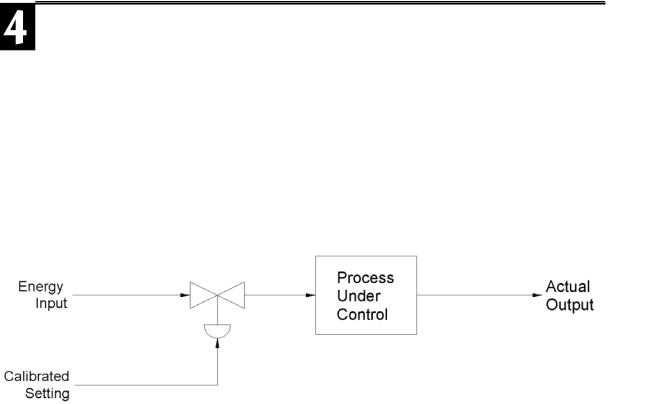
The simplest form of control is open loop. The block diagram in Figure 4.7 represents a basic open-loop system. Energy is applied to the process through an actuator. The calibrated setting on the actuator determines how much energy is applied. The process uses this energy to change its output. Changing the actuator’s setting changes the energy level in the process and the resulting output. If all of the variables that may affect the outcome of the process are steady, the output of the process will be stable.

Figure 4.7: Open-Loop Control

The fundamental concept of open-loop control is that the actuator’s setting is based on an understanding of the process. This understanding includes knowing the relationship of the effects of the energy on the process and an initial evaluation of any variables disturbing the process. Based on this understanding, the output “should” be correct. In contrast, closed-loop control incorporates an on-going evaluation (measurement) of the output, and actuator settings are based on this feedback information.

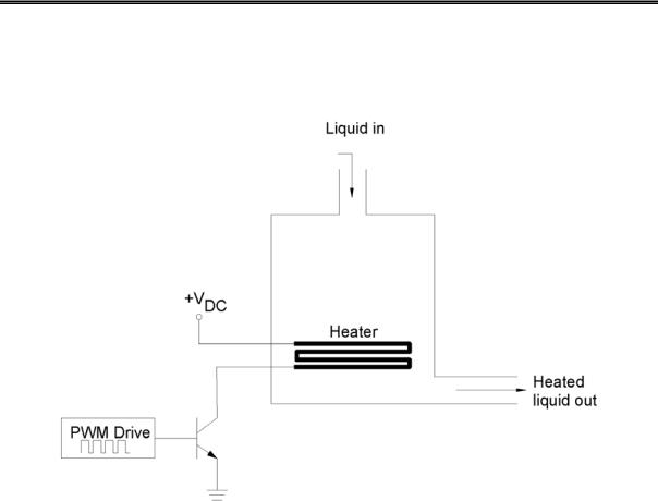
Consider the temperature control process shown in Figure 4.8. The material being drawn from the tank must be kept at a 101o temperature. Obviously, this will require adding a certain amount of heat to the material. (The drive on the transistor determines the power delivered to the heating element.) The question becomes “How much heat is necessary?”

Industrial Control Version 1.1 •Page 113

Experiment #4: Continuous Process Control

Figure 4.8: Open-Loop Heating Application

For a moment, consider the factors that would affect the output temperature. Obviously, ambient temperature is one. Can you list at least three others? How about:

•The rate at which material is flowing through the tank.

•The temperature of the material coming into the tank.

•And, the magnitude of air currents around the tank.

These are all factors that represent BTUs of heat energy taken away from the process. Therefore, they also represent BTUs that must be delivered to the process if the desired output is to be achieved. If the drive on the heating element were adjusted to deliver the exact BTUs being lost, the output would be stable.

Page 114 •Industrial Control Version 1.1

Experiment #4: Continuous Process Control

In theory, the drive level could be set and the desired output would be maintained continuously, as long as the disturbances remained constant.

Let’s now assume that it is your objective to keep the interior of your film canister at a constant temperature. A good real-world example would be that of an incubator used to hatch eggs. To hatch chicken eggs, it is important to maintain a 101oF environment.

Turning on the heater will warm up the interior of the canister. In our earlier test, you turned on the heater’s drive transistor, and the temperature rose above 101oF. Obviously, to maintain the desired temperature, we will not need to have full power applied to the resistor. Through a little testing, you can determine just what drive level would be needed to yield the correct temperature.

The drive to the power transistor in Figure 4.8 is labeled as PWM. This is the acronym for pulse-width modulation. PWM is a very efficient method of controlling the average power to loads such as heating elements. The square wave is driving the transistor as a current-sinking switch. When the drive is high, the transistor is saturated, and full power is applied to the heater. A logic Low applied as base drive puts the transistor in cutoff; therefore, no current is applied to the load. Multiplying the percentage of the total time that the load receives full power times the full power will give the average power to the load. This average ontime is the duty cycle and is usually stated as a percentage. A 50% duty cycle would equate to half of the full power drive, 75% duty cycle is three-quarters full power, etc. It was stated earlier that the 47-ohm “heater” resistor in our canister would receive 1.7 watts when fully powered by the 9-volt unregulated source supply. The pushbutton switch was used to toggle the power on and off. If you were to press the switch rapidly at a constant rate, the resistor would receive 1.7 watts during the ON time and 0 watts during the OFF time. This

50% duty cycle would result in an average power consumption of .85 watts (Paverage = Pfull * duty cycle). Complete the table in Figure 4.9 below for power consumed at duty cycles of 75% and 25% for your system.

Figure 4.9: Average Power

Paverage = Pfull * duty cycle

Industrial Control Version 1.1 •Page 115

Experiment #4: Continuous Process Control

PBASIC provides a useful instruction for providing pulse-width modulation.

Its syntax is: PWM pin, duty, duration

Where: pin is the output pin you are driving.

duty is the duty cycle relative to 255 being 100%.

duration is the window of time in milliseconds over which the duty cycle is provided.

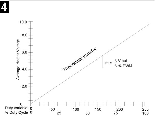
Challenge 2: Graphing PWM duty vs. Vout.

Use your multi-meter to measure the average voltage across the heating element at various PWM commands. Change the duty variable in Program 4.2 to increments between 0 and 255. Plot the average voltage on the graph in Figure 4.10.

'Program 4.2: PWM vs. Vout

'Change the Duty = 50 in increments of 10 between 0 and 100. Measure the

'average output voltage that results.

Page 116 •Industrial Control Version 1.1

Experiment #4: Continuous Process Control

Figure 4.10: Graph of Heater Voltage vs. PWM Duty Cycle

If you are not familiar with PBASIC’s PWM instruction, refer to the BASIC Stamp Manual Version 2.0 pp. 247250. One aspect of using the command should be understood. PWM applies pulses for a period of time defined by the duration value. During the time when the rest of the program is executing, there is no output applied to the load. As a result, the average voltage at a 100% duty cycle (duty =255) will result in a value less than the full voltage expected. The slower your program cycle time, the greater is this disparity. To get a better understanding of cycle time, place a PAUSE 200 in Program 4.2. Compare the resulting output voltage with earlier readings. Change the length of the pause and notice the results.

Recall the Sample and Hold circuit introduced in Challenge #3 of Experiment #2. This circuit held the average PWM voltage across the brushless motor during the entire program loop. This was necessary because of the long program loop and fast response of the fan. The Sample and Hold circuit was effective in delivering the desired average voltage regardless of the program loop-time. In terms of power control, it is more efficient

Industrial Control Version 1.1 •Page 117

Experiment #4: Continuous Process Control

to not use Sample and Hold. This can be understood if you consider driving the circuit at 50%. A 50% drive would result in ½ of the supply voltage appearing across the load continually. This is great. Right? Well if half of the supply voltage is across the load continually, the other half must be across the transistor. This collector- to-emitter voltage times the collector current represents power wasted in the transistor. When system response is fast (like the brushless fan) you have no choice but to use this type of linear power control.

The resistor heating element in our model incubator is a good example of a slow responding system. Straight PWM control of the resistor wastes little power in the transistor because it is only operated in an ON/OFF switching mode. As long as the PWM period is much longer (>10x) than the time required to run the rest of the program loop there will little discrepancy in the Duty cycle and expected average voltage.

Page 118 •Industrial Control Version 1.1