Industrial Control (Students guide, 1999, v1.1 )

Experiment #6: Proportional – Integral – Derivative Control

disturbance is removed providing an error of 10%? It is wise to make a provision in your program to limit the cumulative integral drive to less than 100%

Challenge!

1.What would the system response be if Integral gain were 1 (Ki=10) and the reset time were 60 seconds (Ki=12)? Why?

2.Test and confirm your theory.

Exercise #3: Proportional-Derivative Control

Copid = B +(Kp * E) +(Kd * ∆∆Et )

%DriveTOTAL = %DriveBIAS + %DrivePROP + %DriveDERIV

Derivative control responds to a CHANGE in the error. The fundamental premise determining derivative drive assumes the present rate of change in the error signal will continue into the future unless action is taken. Derivative drive, when properly tuned, allows a system to rapidly respond to sudden changes and react accordingly.

Figure 6.16 illustrates how we would evaluate the slope of an error signal. Finding the difference between error samples taken at regular time intervals reflects the rate at which the process variable is changing. The greater the difference, the greater the slope and therefore the greater the derivative drive necessary to counteract the change.

Industrial Control Version 1.1 •Page 179

Experiment #6: Proportional – Integral – Derivative Control

Figure 6.16: Derivative Error

Consider the act of balancing yourself on a fallen log. Typically you perform slow adjustments to your body position to maintain balance. You are responding proportionally to an error that exists in your equilibrium. Suddenly, a large gust of wind hits you causing you to rapidly loss balance. In response you quickly shift to counteract the wind. This action was based on sudden change in your equilibrium over a very short period of time. In our incubator, a rapid changing temperature will be counteracted by a immediate reduction in drive.

Page 180 •Industrial Control Version 1.1

Experiment #6: Proportional – Integral – Derivative Control

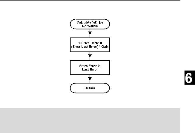
Figure 6.17: Flowchart and Code for Derivative Control

Code for this flowchart:

'*********** DERIVATIVE DRIVE

DerivCalc:

D= (Err-LastErr) * KD ' Calculate amount of derivative drive

'based on the difference of last error

DerivDone

LastErr = Err ' Store current error for next deriv calc

RETURN

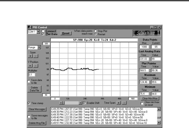
In this experiment, we will repeat the disturbances on a system with a proportional gain of 2 from Exercise #2. Only this time derivative drive will be used in conjunction with proportional. The fan will once again be supplied power from Vin (pin 19) for 10 seconds at 1 inch. Figure 6.18a is the results of our testing. Figure 6.18b is an Excel graph of the data.

1)Settings: Proportional gain of 2 (Kp=20), Ki=0, derivative gain of 1 (Kd=2).

2)Allow temperature to stabilize on SPL.

3)Energize the fan for 10 seconds.

(For this test, our bias temperature was 99.0F)

Industrial Control Version 1.1 •Page 181

Experiment #6: Proportional – Integral – Derivative Control

Figure 6.18a: Disturbance Response with

Proportional Gain of 2 and Derivative Gain of 2

Compare this with Figure 6.9a using only proportional drive. Note that the system stabilizes much faster with fewer oscillations and overshoot. In the message section, there are 2 consecutive reading of 99.0F. First had a %D drive of 40% since there was a 20% error change (.4F) between the previous and current. The second resulted in a %D of 0% because 2 consecutive readings of 99.0F represents no change in error and a slope of zero.

Page 182 •Industrial Control Version 1.1

Experiment #6: Proportional – Integral – Derivative Control

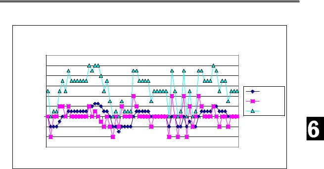
Figure 6.18b: Graph of Data

Note in the above graph how a change in %Err results in a derivative drive. When error is constant, although high, %D is 0. The greater the change in %Err, the greater %D. A positive going %Err (temperature decreasing) results in a positive derivative drive in an effort to stop the change.

Let’s work a little math for a temperature change between samples of 99.4 to 99.0 with the setpoint at 99.0F:

%DriveTOTAL = %DriveBIAS + %DrivePROP + %DriveDERIV

At the time of the first sample, T=99.4:

Error = setpoint – actual = 99.0F-99.4F = -4F %Error = Error/Range * 100 = -.4F/2F * 100 = -20%

Temperature dropped to 99.0F at the time of the second sample:

Error = setpoint – actual = 99.0F-99.0F = 0F %Error = Error/Range * 100 = 0F/2F * 100 = 0%

%DrivePROP = %Error * Kp = 0% * 2 = 0%

%DriveDERIV = (This %Error – Last %Error) * Kd= (0%-20%) * 1 = 40%

Industrial Control Version 1.1 •Page 183

Experiment #6: Proportional – Integral – Derivative Control

%DriveTOTAL = %DriveBIAS + %DrivePROP + %DriveDERIV = 50%+0%+40% = 90%

Even though temperature returned to the setpoint providing a 0% drive from proportional, the temperature dropped from the last reading. Derivative control took action based on the change in error in an effort to stop the dropping temperature by adding drive.

If the next temperature reading was 99.2%, what would the final drive be?

Challenge!

1.What would system response be with a derivative gain of 5? Why?

2.With a -0.3 change in temperature from the setpoint, what would total drive be?

3.Test and confirm your theory.

Proportional-Integral-Derivative Summary

With PID control, 3 separate drive evaluations are performed to calculate the final drive to the control element. Bias drive is used to estimate the drive needed to sustain a setpoint under nominal conditions.

Proportional drive acts by adding an amount of drive in proportion to the amount of error that exists between the setpoint and the actual value. The higher the proportional gain the greater the controller’s response, though overshoot and oscillations are more likely. Some error must exist for proportional drive to act, often resulting in a stable but offset condition.

Integral drive acts by integrating a long error over time and taking action based on the total error. Integral is used to drive away error conditions that persist over a period of time. Integral control is also a good choice for a very slow approach to a setpoint when long system settling times are needed and overshoot is undesirable.

Page 184 •Industrial Control Version 1.1

Experiment #6: Proportional – Integral – Derivative Control

Derivative control acts by taking action based on a change of error, often from one reading to the next. It evaluates the slope of the changing output and acts in opposition to the change. Derivative control can prevent hunting and oscillations, but too much drive can send a system into wild oscillations.

Each control mode has its own unique characteristic response to maintaining the desired output to it, such as response time. Volumes have been written on the subject of PID control and tuning. Tuning a PID system involves adjusting the software parameters for each factor. The goal of tuning the system is to adjust the gains so the loop will have optimal performance under dynamic conditions. As mentioned earlier, tuning is as much of an art as it is a science. The basic procedures for tuning a PID controller are as follows. This procedure assumes you can provide or simulate a quickstep change in the error signal:

1.Turn all gains to 0

2.Begin turning up the proportional gain until the system begins to oscillate.

3.Reduce the proportional gain until the oscillations stop, and then drop it by about 20 % more.

4.Increase the derivative term to improve response time and system stability.

5.Next, increase the integral term until the system reaches the point of instability, and then back it off slightly.

As you gain experience in embedded control, you will see that the characteristics of the process will determine how you should react to error. Consider the following three real-world applications.

What are the important characteristics of these processes that will determine the suitable control scheme? What mode(s) of control do you feel would work the best?

1)Similar to our incubator system, the first application is a home project that uses the LM34 to

measure the temperature of a 20-gallon aquarium. Water temperature is maintained within + 1 degree of 80 oF by varying the duty cycle of a 200-watt heater. Room temperature varies from 65 to 75 degrees.

2)The second application controls the acidity (pH) in the production of a cola soft drink. The plant’s water supply has a pH of 7.2 to 7.4. The flow stream of water into a batch of soda must be maintained at a pH of 6.8. An upstream valve is opened accordingly to release phosphoric acid into the stream. The pH sensor is relatively slow. The amount of acid needed varies with incoming pH and water flow rate.

3)In a plant science research facility at San Diego State University, the surface temperature of a plant’s leaf must be held constant. The plant is contained in a small (shoebox sized) greenhouse. A

Industrial Control Version 1.1 •Page 185

Experiment #6: Proportional – Integral – Derivative Control

very fast thermocouple sensor rests on the leaf and measures temperature. Disturbances such as changes in wind, sunlight, and plant metabolism can happen quickly and in high magnitudes.

We have just scratched the surface of process control theory through feedback. Our focus has been limited to control action based on feeding back information from the output of our process. When disturbances affect our process, changes in the output are detected and generate an error signal. PID is tuned to drive the error away as quickly as possible. Tight control of the process variable is possible with PID, but the fundamental premise of feedback control is to respond to error. Error is expected and, to a certain degree, tolerated. As we leave this chapter, consider an alternative to feedback control. That is feed-forward control. In feedforward control you measure those factors that disturb a process. Understanding how they affect the variable we are holding constant will allow for output action to be taken before an error signal results. If you could measure changes in ambient temperature and wind speed from the fan, could you use this information to better control our incubator? Interesting concept isn’t it?

Page 186 •Industrial Control Version 1.1

Experiment #6: Proportional – Integral – Derivative Control

Questions and Challenge

1.Would on/off control of the system be suitable for PID control? Explain.

2.Which type of control (proportional, integral, or derivative) would be best suited for the following?

a.To return a system to the setpoint based on the difference between Actual temperature and the setpoint due to a short-lived disturbance: ________________.

b.To minimize the effect that a quick disturbance has on the system: ______________.

c.To reduce the effect that a long-term disturbance has on the system: ______________.

3.A system has a setpoint of 101.5 degrees, and an allowable band of +/- 0.5 degrees. For a 50% proportional band, what would be the proportional gain? ____________.

4.A system has a setpoint of 101.5 with a gain of 3. If the Actual temperature were 101.2, what would be the drive due to proportional error? ___________

5.A system has a derivative gain of 2. If the temperature dropped from 101.8 to 101.3 between readings, with a setpoint of 101.5, what would be the error due to derivative drive? __________.

Industrial Control Version 1.1 •Page 187

Experiment #6: Proportional – Integral – Derivative Control

Final Control Challenge

From a cold condition (incubator at room temperature), find the values of PID control which will bring the incubator to an operating temperature of 95 degrees the quickest with minimal overshoot and hunting. Graph and record your results (note the graph scales):

Kp=____ Ki=____ Ti=____ Kd = ____

Time first reached 95.0F: _________

Maximum value reached: (Time)_________ (Value) __________

Next minimum reached: (Time)__________ (Value) ___________

Capture a screen shot (ALT-Prt Scrn) and print using MS Paint.

Find a system:

Find an example of a system that either does or could employ PID control. Discuss how PID control may be implemented to control it.

Alternative Systems to maintain:

1.Use the sample and hold circuit (Figure 2.17) from Experiment #2. Physically connect the heater and sensor with an appropriate material (non-conductive and can withstand the heat). Change the PWMtime 1 because of the much smaller mass and holding of output. Find the 50% bias temperature and attempt to regulate using PID control.

2.Use the output of Pin 8 (drive output without the sample and hold) to drive a solid-state relay controlling a lamp. Place lamp and sensor in an appropriate container. Regulate temperature in this larger incubator system.

Page 188 •Industrial Control Version 1.1