Industrial Control (Students guide, 1999, v1.1 )

Experiment #6: Proportional – Integral – Derivative Control

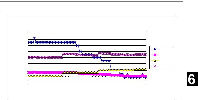
Figure 6.9b: Data File Plotted in Excel

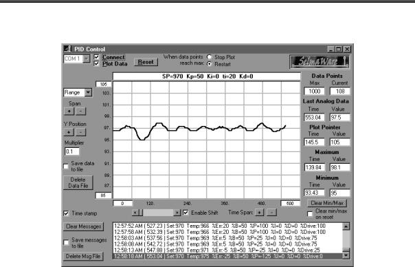
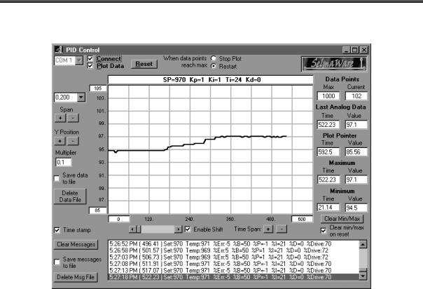
From Figure 6.9b note that at this gain setting the amount of proportional drive (%P) is twice as much as the error (%Err).

Verify the drive amounts shown in the message window of Figure 6.7a at 96.7F:

PID Control: 20% Proportional Band, Proportional Gain = 5

Too much gain can be unsuitable for control. Repeat the experiment for a proportional band of 20% at a gain setting of 5. Kp = 50 in the control settings. Figure 6.10 is our SPL result.

Industrial Control Version 1.1 •Page 169

Experiment #6: Proportional – Integral – Derivative Control

Figure 6.10: Response with Gain = 5, 20% Band

Note that the response time of the system is again slightly faster, but there is much more hunting and continued instability in the system.

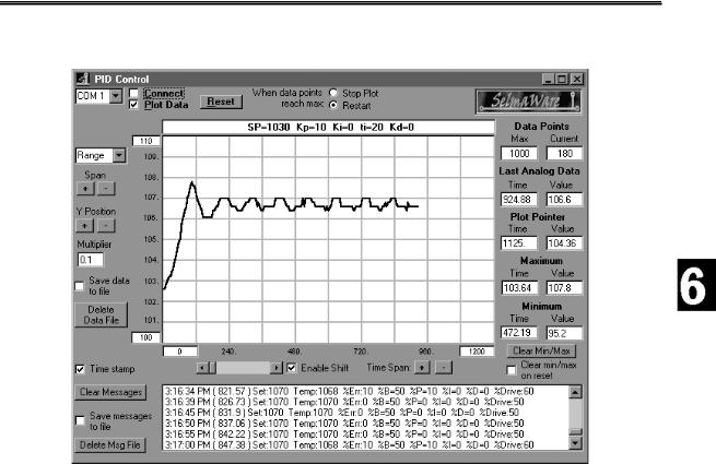
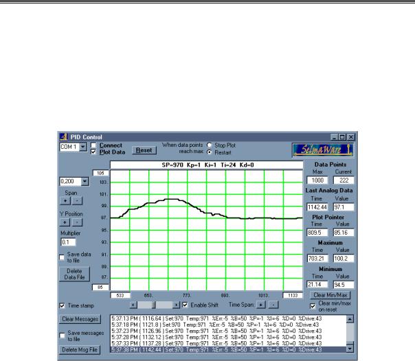
As a final experiment, set the setpoint (SP) temperature substantially higher than the bias temperature, but within a controllable temperature range with a proportional gain of 1 (Kp=10). We tested at 10F above the bias temperature (107F). Plot the results. Figure 6.11 is the result of our tests.

Page 170 •Industrial Control Version 1.1

Experiment #6: Proportional – Integral – Derivative Control

Figure 6.11: Setpoint 10F (107F) above Bias Temperature

While trying awfully hard, the temperature is not stabilizing at 107 degrees. If 107F is an achievable temperature for the system, why doesn’t it stabilize there? Remember that for our system 50% drive stabilized around 97F. Additional drive is added because an error exists. If the incubator were able to stabilize at the setpoint, the error would be 0, providing 0% drive from proportional and only bias drive that is insufficient to maintain the temperature creating an error.

%DriveTOTAL = %DriveBIAS + %DrivePROP

%DrivePROP = Kp*E. If E = 0 then %DrivePROP = 0%. %DriveTOTAL = 50% + 0%

If the setpoint temperature is not the bias temperature, some error MUST exist to provide additional drive from the proportional control. The higher the proportional gain, the smaller the remaining error. In the next section, we will see how Integral Error may be used to drive away this remaining error.

Industrial Control Version 1.1 •Page 171

Experiment #6: Proportional – Integral – Derivative Control

Challenge!

1.If the proportional gain were set to .5 (Kp=50), what type of response would you expect from the system? Why?

2.If the temperature is 0.6F below your setpoint, what would the total drive be?

3.Confirm your theory.

Exercise #3: Proportional+Integral Control

Copid = B +(Kp * E) +(Ki * ∫Et)

%DriveTotal = %DriveBIAS + %DrivePROP + %DriveINT

So far we’ve looked at what occurs when quick disturbances occur to our system in equilibrium. Proportional control may be used to drive the temperature back to the desired setpoint. But what happens when the disturbance affects the equilibrium of our system over a long period of time? At the end of the last experiment it was seen what occurs when the bias drive is not sufficient to make-up for average losses. Because some error must exist for proportional drive, the setpoint temperature cannot be maintained.

Integral control can be used to drive-away error remaining due to long lasting disturbances in the system. These may be from additional losses or gains of energy that remain for a long period of time. Consider our incubator. We found a bias temperature at which a 50% bias drive was sufficient to make up for the losses in the system maintaining it in equilibrium.

But what would happen if the fan were continuously pointed at the incubator? Continuous system losses would be higher. The 50% bias drive will be insufficient to maintain the temperature and proportional drive will respond to the error in an attempt to drive the system back toward to the setpoint. But as we’ve seen, because some error must remain, the setpoint is not maintained. The system will stabilize at a temperature below the desired setpoint.

Over time, integral drive can be used to drive away this error, allowing the temperature to reach the setpoint.

Integral drive is also used when a slow approach with long stabilization times are needed to ensure no overshoot. Consider the example of cooking soup. After cooking a bit, you taste, add an amount of salt you feel appropriate for what you would like the final taste to be. Do you taste immediately and add more? No, you wait a while to allow the salt to blend in, then taste, and add a bit more until you finally reach your desired taste. What if too much salt is added? Cutting back is a bit more difficult!

Page 172 •Industrial Control Version 1.1

Experiment #6: Proportional – Integral – Derivative Control

An industrial example may be that of adding pigment to paint for a desired color. Electronic circuitry monitors paint color and gradually add pigment until the desired color is reached.

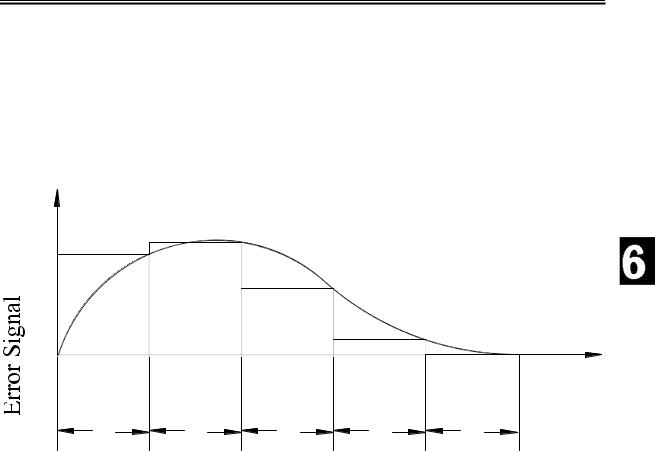
In integral drive the amount of error is integrated over time. The larger the error and the longer it lasts, the greater the integral drive will be.

As seen from figure 6.12, the amount of error under the curve is added together to find the integrated error. The longer the error exists, the higher integrated total error (ET) will be.

Figure 6.12: Integrating Error

The integrated error is multiplied by the integral gain to find the integral drive.

ET = Σ(E1+E2+E3+…)

%DriveINT = Ki* ET/T

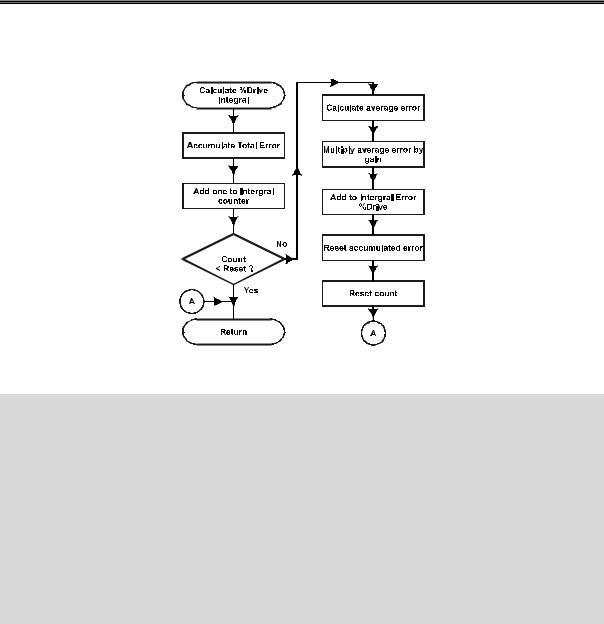
How often should the integral gain be updated or reset? Integral drive should be based on stabilized readings. Depending on the response time of the system this may be anywhere from seconds to hours or even days. Just as with adding salt to the soup, if system hasn’t stabilized from the last addition, it would be easy to add too much. The stabilization time of our incubator was found back in Experiment #1 of this section and was 450 seconds for our testing. Figure 6.13 is the flowchart for the integral calculations.

Industrial Control Version 1.1 •Page 173

Experiment #6: Proportional – Integral – Derivative Control

Figure 6.13: Integral Flowchart

Code to accompany chart above:

RETURN

Page 174 •Industrial Control Version 1.1

Experiment #6: Proportional – Integral – Derivative Control

Controlling the Incubator

In this exercise, the fan will be used to produce a long lasting disturbance to the system. The fan should be placed approximately 6 inches from the incubator. It will be powered from Vdd (5V – Pin 20 or from the Vdd terminal on top of the breadboard) to provide a ‘gentle’ cooling to the canister (you may have to ‘kick-start’ the fan to start it turning). This will produce a long-term disturbance to the system instead of the strong 10 second disturbances used in the proportional testing.

For proportional gain we will use a very small value to prevent hunting and provide a large error from the setpoint. The integral update time, or reset time, of the integral drive will be approximately 120 seconds (450 seconds would be more appropriate to allow full stabilization, but that’s a long time to plot!). Integral gain will be set in tenths.

1)Setup Program 6.1 for a 1000% Proportional Band, Gain of 0.1 (Kp=1) and Integral gain of 0(Ki=0) and derivative of 0 (Kd=0).

2)Point the fan at the incubator from a distance of about 6 inches (if you see no response after 30 seconds, move it closer in one-inch increments and try again).

3)Energize the fan from Pin 20 (5V) and ground. Push-start the fan if needed.

4)Allow the system to stabilize with this new system loss.

5)Change the integral gain to .1 (Ki=1), Ti = 24.

6)Download and plot at the new settings.

Figure 6.14a shows our results of this test with a bias setpoint of 97.0 F and Figure 6.14b is an Excel plot of captured data.

Industrial Control Version 1.1 •Page 175

Experiment #6: Proportional – Integral – Derivative Control

Figure 6.14a: Long-Term Disturbance Effects

Note that with a bias setpoint of 97.0F and the disturbance of the fan, the initial stable temperature was 94.8F. Over time the drive, and hence the temperature, was slowly bumped up until the actual temperature was at the setpoint.

Page 176 •Industrial Control Version 1.1

Experiment #6: Proportional – Integral – Derivative Control

Figure 6.14b: Data Plotted in Excel

Note that the initial error (%Err) was 11% at a stable temperature of 94.8F.

%DriveTotal = %DriveBIAS + %DrivePROP + %DriveINT %DrivePROP = Kp * ET = 0.1 * (97.0F-94.8F)/2F * 100 = 11% %DriveINT = Ki * 0 until the first reset time.

%DriveTotal = 50% + 11% + 0%

Around 120 seconds, the first integral reset time occurs. All the error samples prior to that time are summed and averaged over time. This is multiplied by the integral gain to find the integral drive.

%DrivePROP = 11% still since the temperature is still 95.8F

%DrivePROP = Kp * ET = .1 * (11%+11%+11%….[24 of them!])/24 = 11% %DriveTotal = 50% + 11% + %11% = 72%

Note that with the higher total drive (%Drive), temperature eventually begins to increase, error decreases, and proportional drive decreased. Integral remains constant until the next reset time around 240 seconds when it bumps up based on the average of the errors since the last reset time.

Eventually, temperature returns to the setpoint, the error is driven away, proportional drive is virtually gone and integral drive plus the bias drive are maintaining the temperature.

Industrial Control Version 1.1 •Page 177

Experiment #6: Proportional – Integral – Derivative Control

%DriveTotal = %DriveBIAS + %DrivePROP + %DriveINT %DriveTotal = 50% -1% + 21% = 70%

But what happens when the long lasting disturbance leaves?

1)De-energize the fan.

Figure 6.15: Temperature Following the Removal of a Disturbance

Figure 6.15 shows what happens when the disturbance is removed. The additional drive from integral drive must be slowly integrated away again.

Integral wind-up can occur if the addition of integral drive is insufficient to force the system back to the setpoint. Integral drive would continually be added. This would mean that an error would constantly persist and the output would ‘wind-up’ to an abnormally high values leading to an unresponsive system. If our program allowed integral drive to wind-up to 20000%, how long would it take to drive it away once a

Page 178 •Industrial Control Version 1.1