Industrial Control (Students guide, 1999, v1.1 )

Experiment #4: Continuous Process Control

Challenge #3: Analyzing your Open-Loop System

The following program is developed to study the relationship between PWM drive on your heater and the resulting stable temperature. The program will apply PWM drive levels in 10% increments. Each increment will last approximately four minutes. The program will end after 100% drive has been applied. StampPlot Lite will give you a graphical representation of your system’s response, along with time stamp information in the list box. Furthermore, if you are really interested, the StampPlot Lite data file can be imported into a spreadsheet, applied to a graph and analyzed.

Figure 4.11: Screen Shot of PWM Drive vs. Temperature

Industrial Control Version 1.1 •Page 119

Experiment #4: Continuous Process Control

Figure 4.11 is typical of a StampPlot Lite screen shot resulting from this test. Load Program 4.3. Before running the program, be sure your canister has cooled to room temperature. Place the cap on your canister and start the program. When the DEBUG window appears, close it and start StampPlot Lite. Connect using StampPlot Lite and press the restart button to reload the program and begin the test.

Page 120 •Industrial Control Version 1.1

'Get and display initial starting values.

GOSUB Getdata GOSUB Calc_Temp

DEBUG "Temp = ", DEC Temp, " Duty = ", DEC Duty,CR

DEBUG "!USRS Begining Test! -- Testing at ", DEC Drive, "% Drive.",CR

DEBUG "!USRS Testing at ", DEC Drive, "% Drive",CR

Industrial Control Version 1.1 •Page 121

Experiment #4: Continuous Process Control

Tick = 0

Page 122 •Industrial Control Version 1.1

Experiment #4: Continuous Process Control

Challenge #4: Open-Loop Control--Desired Setpoint = 101o Fahrenheit

It is our objective to maintain a constant canister temperature of 101o Fahrenheit. Follow these procedures. Record values in the table of Figure 4.12.

1. Study the StampPlot Lite analysis that resulted from running Program 4.2. From the Text Box listing, record in the table the beginning ambient temperature, the temperature at the end of the 50% drive test, and the ending maximum temperature after 100% drive.

2. Use your cursor to find the Drive level that resulted in a temperature of 101 degrees.

3. Next, modify the Control subroutine of Program 4.2 so that the duty cycle remains at the constant value declared initially. Do this by removing the two lines indicated below.

4. At the beginning of the program, declare the DutyCycle to be the value that yielded 101o in our test StampPlot Lite. Run the program and allow the system to stabilize. How close was your estimation? Bump it up or down accordingly to find the setting that yields the desired result. In line #5 of the table, record the percent of drive that places the system at or near 101 degrees. Let it run for a moment and take note of the system stability. Once a drive setting has been established, an open-loop system will stabilize; and, as long as the disturbances that affect the process stay constant, so will the output.

5. Plug in the brushless fan across the Vdd supply and aim it directly toward the canister. The moving air represents a change in the disturbance on your process. According to theory, heat will be removed from the process at a greater rate and the new stable temperature will be lower than 101o. With the fan blowing on the canister, try to find the new “correct” drive for this condition. Record your data in line #6 of the table.

Industrial Control Version 1.1 •Page 123

Experiment #4: Continuous Process Control

Figure 4.12: Open-Loop Control Table

6.Finally, leaving the proper setting established in line #6, change the position of the fan so it is blowing less directly on the canister. This represents a medium disturbance level on the system. Assess the situation and make your best guess as to the proper drive setting required by this new condition. Program the BASIC Stamp for this drive level. Once the system stabilizes, record your results in line #7 of the table.

Challenge #5: Determining an Open-loop Setting

1.Select a new “desired temperature” for your system. Predict and program an open-loop drive value that will maintain this temperature.

2.Place a couple of glass marbles in your canister. See how increasing the mass of the system affects the response and the drive setting necessary to maintain the new condition. What conclusions can you draw from the system’s behavior?

There are many variables that can affect the relationship of drive level and temperature in your small environment. Given some time to experiment and become familiar with the dynamic relationship between temperature, drive level, and disturbances, you could get pretty good at assessing the conditions and setting the right amount of drive in an open-loop manner. As we see, however, if any condition of our process changes, so will the output. Open-loop control can be useful in some applications. When a process requires that its output remain constant for all conditions, then closed-loop control must be employed. In closed-loop control, action is taken based on an evaluation of the measurement and the desired setpoint. This evaluation results in what is called an “error signal.” Experiment #5 and #6 will guide you through 5 modes of closedloop control.

Page 124 •Industrial Control Version 1.1

Experiment #4: Continuous Process Control

Questions and

Challenge

1.Give two examples of continuous process control other than those given in the text.

2.How is the drive level in open-loop control determined?

3.What is the primary advantage of open-loop control?

4.What is the primary disadvantage of open-loop control?

5.The ADC0831 will convert a range of analog input to one of 256 possible binary values. The number 256 identifies the _________ of the converter.

6.The purpose of the chip select and clock lines to the ADC0831 are to ____________ the conversion process.

7.If the LM34 were placed in a 98.6-degree environment, the expected output would be _________volts.

8.In pulse-width modulation, the amount of drive action is based on the __________ of time ON over the total time.

9.If a 40-watt heater were pulse-width modulated at a 75% duty cycle, the average power consumed would be __________ watts.

10.When disturbances change in an open-loop process, so does the ____________.

Challenge: Open-loop Control of the Fan

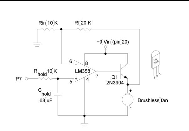
Recall in Experiment #2, the circuit in Figure 4.13 was introduced to control the speed of the brushless motor fan.

Industrial Control Version 1.1 •Page 125

Experiment #4: Continuous Process Control

Figure 4.13: Sample and Hold PWM Drive

Because of the fan’s quick response to voltage fluctuations, the Sample and Hold circuit is necessary to effectively control speed using the PWM instruction. Construct this circuit to be able to vary fan speed. Directly connect the resistor across the +Vin supply. With the fan directly pointed toward the canister, experiment with different PWM drive levels to the fan. What drive level is necessary to cool the canister to 101oF?

Page 126 •Industrial Control Version 1.1

Experiment #5: Closed-Loop Control

An open-loop control system can deliver a desired output if the process is well understood and all conditions affecting the process are constant. However, Experiment #4 showed us that an open-loop control system couldn’t guarantee the desired output from a process that was subject to even mild

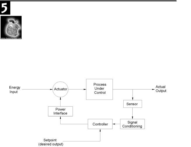
disturbances. There is no mechanism in an open-loop system to react when disturbances affect the output. Although you were able to find a drive setting that would yield the desired temperature in Experiment #4, when the fan was moved closer or further from the heater, the fixed setting was no longer valid. Closed-loop control provides automatic adjustment of a process by collecting and evaluating data and responding to it accordingly. A typical block diagram of an automatic control system is depicted in Figure 5.1.

Figure 5.1: Closed-Loop Control

In this diagram, an appropriate sensor is measuring the Actual Output. The signal-conditioning block takes the raw output of the sensor and converts it into data for the Controller block. The Setpoint is an input to the Controller block that represents the desired output of the process. The controller evaluates the two pieces of data. Based on this evaluation, the controller initiates action on the Power Interface. This block provides the signal conditioning at the controller’s output. Experiment #3 discussed several methods of driving power interface circuits. The Power Interface has the ability to control the Actuator. This may be a relay, a solenoid valve, a motor drive, etc. The action taken by the Actuator is sufficient to drive the Actual Output toward the desired value.

Industrial Control Version 1.1 •Page 127

Experiment #5: Closed-Loop Control

As you can see, this control scenario forms a loop, a closed-loop. Furthermore, since it is the process’s output that is being measured, and its value determines actuator settings, it is a feedback closed-loop system. The

The type of reaction that takes place upon evaluation of the input defines the process-control mode. There are five common control modes. They are on-off, on-off with differential gap, proportional, integral, and derivative. The fundamental characteristic that distinguishes each control mode is listed below in Table 5.1.

Table 5.1: Five Common Control Modes

Continue taking more forceful action for the duration the error exists.

This exercise will focus on converting the open-loop temperature control system of Experiment #4 into an on-off closed-loop system. Our system will show advantages and disadvantages to this method of control. The characteristics of the system being controlled determines how suitable a particular control mode will be. Experiment #6 will use the same circuitry to overview and apply proportional, integral, and derivative control modes. Leave the circuit constructed after completing this step.

Figure 5.2 is a schematic of the circuitry necessary for the next two exercises. As you see, this is identical to Experiment #4. The 35-mm film canister provides the environment we wish to control. The heater drive provides full power for developing heat in the resistor. The LED is also driven by Pin 8. Remember that the LED is driven by the +5-Vdd supply, and the heater is driven by the +9-volt unregulated line supply. The LM34 sensor will provide temperature data. In closed-loop control, we will monitor the temperature and use it to determine control levels. The fan’s air currents will act as a disturbance to the process.

Page 128 •Industrial Control Version 1.1