Industrial Control (Students guide, 1999, v1.1 )

Run the program and observe the behavior of your system.

Challenge! Observe and Evaluate Differential-Gap Control

Allow the program to cycle a few times. Report on the following:

Record the minimum and maximum overshoot temperatures.

Maximum overshoot _______________ Minimum Overshoot __________________

With your cursor, investigate time between cycles. Record these times below.

Industrial Control Version 1.1 •Page 139

Experiment #5: Closed-Loop Control

Project the switching point of the digital output down to the plotted temperature. Can you determine the temperature at which switching occurred? Momentarily remove the 10-uF filter capacitor. Does the increase in noise cause rapid cycling about the limits?

Use the fan to change the disturbances to the process. Reset the program and watch the control action. Describe any effect the new level of disturbance has on the overshoot and/or the cycling. Summarize how you have changed the dynamics of your system.

Place a single glass marble in the canister. Restart the program and summarize how increasing the mass has affected the process control action. Investigate the cycle time and overshoot.

Simple ON/OFF or Differential Gap?

Hopefully, the data that you have observed and recorded will reveal some important characteristics of these two control modes. They both have advantages and disadvantages. Simple on-off control results in rapid cycling of the heating element. Reported cycle times of less than one second could easily result if your system has fast recovery or there is noise on the analog line. Rapid cycle time would not be acceptable if our heater were being controlled by an electromechanical relay.

Notice, however, that the overshoot is approximately a half-degree and our average temperature is at the desired setpoint. Compare this control response to that observed when Differential Gap has been added to the On/OFF control.

With Differential-Gap control, you will notice fundamental differences in the control action.

1.Rapid cycling about the setpoint no longer occurs.

2.The minimum and maximum values still overshoot, but now beyond the limits.

3.Total cycle time between ON/OFF conditions is longer.

Increased cycle time and noise immunity about the setpoint are definite improvements over simple on-off control. The tradeoff, however, is allowing the process to vary further from the desired temperature setpoint. Obviously, an understanding of your process and its hardware will determine the appropriate control mode.

Page 140 •Industrial Control Version 1.1

Experiment #5: Closed-Loop Control

Both modes took appropriate control action to maintain temperature under changing disturbance levels and load conditions. The drawback to either mode of ON/OFF control is that the controlled variable is constantly on the move. The fully-ON and fully-OFF conditions of the final control element are continually forcing the measurement past the limits.

If you recall, in the Open-Loop Control exercise of Experiment #3, a value of drive between off and fully on was found to be appropriate to hold the temperature at the setpoint. If all disturbances to the process remained constant, the temperature would stay at the setpoint when the right percentage of drive was applied. We also saw that as conditions changed, so did the measurement. Experiment #6 will investigate controls that take an appropriate amount of action based on an evaluation of the measurement. Applying Proportional, Integral, and Derivative control theory can be employed to maximize the effectiveness of the control system.

Programming Challenges

1.Alter your program so a +1 degree differential gap can be calculated automatically, based on the desired setpoint.

2.Add a variable called Differential_gap so the operator needs only to enter the Setpoint and the amount of Differential gap and the program automatically performs the desired action.

Industrial Control Version 1.1 •Page 141

Experiment #5: Closed-Loop Control

Questions and Challenge

1.Write one complete sentence that clearly states the fundamental difference between Open-loop and Closed-loop controls.

2.Simple ON/OFF control compares the measurement of the process variable to a

________________.

3.If the final control element to our model incubator were an air conditioner instead of a heater, what would change about Program 5.1?

4.When the process variable continues to increase after the final control element is turned OFF, it is termed _______________.

5.Rapid cycling about the setpoint of an ON/OFF control system is a result of __________ riding on the measurement data.

6.List three devices that could not withstand rapid cycling of power.

____________________

____________________

____________________

7. Process cycle time is directly affected by the amount of ____________ in the system.

Page 142 •Industrial Control Version 1.1

Experiment #5: Closed-Loop Control

8.Differential-gap control takes full action when the process variable crosses the ___________

points.

9.Cycle time will be ______________ if differential-gap control is used in a system rather than simple ON/OFF control.

10.Rapid cycling is not a problem in differential-gap control if the measurement data plus the

___________ is less than the differential gap.

11.When the measurement is between the limits, the output will be in the mode determined by which limit was exceeded __________.

12.Adding more mass to a Differential-gap control system will ___________ the amount of overshoot and ___________ the cycle time of the process.

Control Challenge: Reverse the Scenario

Reverse the positions of the output devices in Figure 5.2. Replace the heater in figure 5.2b with the brushless fan and place the heater across the +9V supply as shown in Figure 5.2c. Control the temperature by turning the fan on and off while the heater is on all of the time. You will have to change the code to such that the output turns on to drive temperature down and off as temperature falls below the setpoint. You may want to place the heater and sensor closer together and open the end of the canister to be able to blow air directly onto the pair. This will change the dynamics of the system. It may cycle faster, perhaps overshoot less, and be more susceptible to chatter. Experiment with it and note your observations. Realize that every system that you work with will have its own unique dynamic characteristics.

Industrial Control Version 1.1 •Page 143

Experiment #5: Closed-Loop Control

Page 144 •Industrial Control Version 1.1

Experiment #6: Proportional – Integral – Derivative Control

One objective of a process control is to hold a system constant. In the previous exercise, we used various means of cycling the heater of our incubator to maintain a desired temperature. Using differential gap, we created an allowable band in which the heater would cycle, causing the temperature to cycle above and below the setpoint. In Experiment #4, we saw how we could use pulse-width modulation (PWM) to add energy to our system in duty cycles between 0% (fully off) and 100% (fully on). While these types of control had their advantages and disadvantages, PID control allows the greatest control of a system but can be more difficult to implement and tune (or adjust) for optimum performance.

Holding a process constant involves continually adding energy that equals the system’s losses exactly. If the system’s losses were constant, the process control would be as simple as applying one steady state level of drive. However, the factors that affect a process do change. They change in unpredictable magnitudes and at unpredictable rates. Compounding this problem is that a system has reaction delays that must be understood. An instant change in losses due to a disturbance is not felt immediately, and the change in drive to a system is not either. Process control can be as much an art form as it is a science.

The first step to understanding PID control is that every system has both gains and losses of energy.

Esystem = Ein–Eout

A system is said to be in equilibrium when the energy gained equals the energy lost.

Equilibrium: Ein = Eout

When in equilibrium our incubator would maintain a constant temperature. But this is seldom, if ever, the case. Depending on the heater drive and conditions surrounding the incubator, temperature will either be increasing or decreasing. As conditions change, such as room temperature changing, air movement changes on the canister, sunlight falling on the canister, or the resistor aging, the amount of heat added and removed is seldom constant.

Industrial Control Version 1.1 •Page 145

Experiment #6: Proportional – Integral – Derivative Control

Consider other examples of systems, such as an oil-flow system. The drive element, the pump, is controlled to maintain a desired oil flowrate. A sudden change in the system may be a valve being shut blocking one path for oil flow. Slow change in the system may be corrosion of the piping causing friction or the changing of the oil temperature. The pump needs to adjust in order to compensate for these losses.

One other system to consider is an automobile. Typically we want the car to maintain a constant speed on the highway. The engine makes up for friction losses from the tires on the pavement and wind losses. When the car is maintaining a constant speed, the system is in equilibrium and our foot keeps the accelerator in constant position. When conditions change, such as the car climbing a hill, the cars velocity changes and it begins to slow. The force of gravity increases on the car and these increased losses remove more energy than the engine is supplying and the car begins to slow. Without depressing the accelerator more will the car eventually come to a stop on the hill? No, it will slow to a lower constant speed where once again losses = gains and a new equilibrium is reached.

Conditions, or disturbances on our system, can change very rapidly, such as when a gust of air suddenly blows over the incubator or very slowly such as the heating element aging. PID control can measure and take action on:

1)How far from the setpoint a system is, or the magnitude of the error.

2)The duration that an error remains.

3)How quickly an error occurs in the system, or the rate of change.

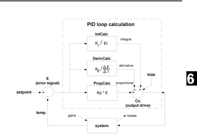
The sums of these three evaluations comprise the output drive in an attempt to maintain a system in equilibrium. Figure 6.1 illustrates the evaluation and control of a system for PID control.

The classic PID formula for calculating the controller output is as follows:

∆E Copid = (Kp * E) +(Ki * ∫Et) +(Kd * ∆t )

Where:

Co = controller output or drive Kp = proportional gain

E = error signal Ki = integral gain

Kd = derivative gain

The drive equation based on the above is:

%DriveTotal = DrivePROP + DriveINT + DriveDERIV

Page 146 •Industrial Control Version 1.1

Experiment #6: Proportional – Integral – Derivative Control

Figure 6.1: PID Control Block Diagram

In this section, the incubator will be controlled using PID control and the PID equation will be explored and illustrated.

Circuit Construction

We will use the same circuit from Exercise #5 (Figure…), but you will manually connect the fan to Pin 19 Vin power or regulated 5V when needed for a disturbance.

The following is the full program for this section. We will change values in the PID Control Settings in testing the different areas of control.

Industrial Control Version 1.1 •Page 147

Experiment #6: Proportional – Integral – Derivative Control

'Program 6.1: PID Control with the StampPlot Interface '********* PID CONTROL SETTING ****************

Page 148 •Industrial Control Version 1.1