Добавил:

PavelEngineer Опубликованный материал нарушает ваши авторские права? Сообщите нам.

Вуз:

Севастопольский Государственный Университет

Предмет:

[НЕСОРТИРОВАННОЕ]

Файл:

[James_Stewart]_Single_Variable_Calculus_Early_Tr(BookFi).pdf

Скачиваний:

Добавлен:

30.12.2019

Размер:

18.09 Mб

Скачать

☆

<<< < Предыдущая 1 2 3 4 5 6 7 89 / 919 10 11 12 13 14 15 16 17 18 19 20 21 22 23 24 25 > Следующая >>>

(b) t$x# ! x2

(d) j$x# ! x4

CHAPTER 1 REVIEW |||| 73

1 R E V I E W

C O N C E P T C H E C K

1.(a) What is a function? What are its domain and range?

(b)What is the graph of a function?

(c)How can you tell whether a given curve is the graph of a function?

2.Discuss four ways of representing a function. Illustrate your discussion with examples.

3.(a) What is an even function? How can you tell if a function is even by looking at its graph?

(b)What is an odd function? How can you tell if a function is odd by looking at its graph?

4.What is an increasing function?

5.What is a mathematical model?

6.Give an example of each type of function.

(a) Linear function	(b)	Power function
(c) Exponential function	(d)	Quadratic function
(e) Polynomial of degree 5	(f)	Rational function

7.Sketch by hand, on the same axes, the graphs of the following functions.

(a) f $x# ! x

8. Draw, by hand, a rough sketch of the graph of each function.

(a) y ! sin x		(b) y ! tan x
(c) y ! ex		(d) y ! ln x
(e) y ! 1"x		(f) y ! & x &
(g) y ! s	x	(h) y ! tan!1x

9.Suppose that f has domain A and t has domain B.

(a) What is the domain of f $ t?

(b)What is the domain of f t?

(c)What is the domain of f"t?

10.How is the composite function f " t deﬁned? What is its domain?

11.Suppose the graph of f is given. Write an equation for each of the graphs that are obtained from the graph of f as follows.

(a)Shift 2 units upward.

(b)Shift 2 units downward.

(c)Shift 2 units to the right.

(d)Shift 2 units to the left.

(e)Reﬂect about the x-axis.

(f)Reﬂect about the y-axis.

(g)Stretch vertically by a factor of 2.

(h)Shrink vertically by a factor of 2.

(i)Stretch horizontally by a factor of 2.

(j)Shrink horizontally by a factor of 2.

12.(a) What is a one-to-one function? How can you tell if a function is one-to-one by looking at its graph?

(b)If f is a one-to-one function, how is its inverse function

f !1 deﬁned? How do you obtain the graph of f !1 from the graph of f ?

13.(a) How is the inverse sine function f $x# ! sin!1x deﬁned? What are its domain and range?

(b)How is the inverse cosine function f $x# ! cos!1x deﬁned? What are its domain and range?

(c)How is the inverse tangent function f $x# ! tan!1x deﬁned? What are its domain and range?

T R U E - F A L S E Q U I Z

Determine whether the statement is true or false. If it is true, explain why. If it is false, explain why or give an example that disproves the statement.

1.	If f		is a function, then	f $s $ t# ! f $s# $ f $t#.
2.	If	f $s# ! f $t#, then s ! t.
3.	If	f	is a function, then	f $3x# ! 3f $x#.
4.	If x1 % x2 and f is a decreasing function, then f $x1 # ' f $x2 #.

5.A vertical line intersects the graph of a function at most once.

6.If f and t are functions, then f " t ! t " f .

1 7. If f is one-to-one, then f !1$x# ! f $x# .

8.You can always divide by ex.

9.If 0 % a % b, then ln a % ln b.

10.If x ' 0, then $ln x#6 ! 6 ln x.

	If x ' 0 and a ' 1, then		ln x	!ln	x
11.						.
			ln a		a
12.	tan!1$!1# ! 3""4
13.	tan!1x !	sin!1x
		cos!1x

74 |||| CHAPTER 1 FUNCTIONS AND MODELS

E X E R C I S E S

1.Let f be the function whose graph is given.

(a)Estimate the value of f $2#.

(b)Estimate the values of x such that f $x# ! 3.

(c)State the domain of f.

(d)State the range of f.

(e)On what interval is f increasing?

(f)Is f one-to-one? Explain.

(g)Is f even, odd, or neither even nor odd? Explain.

y
	f
1
1	x

2.The graph of t is given.

(a)State the value of t$2#.

(b)Why is t one-to-one?

(c)Estimate the value of t!1$2#.

(d)Estimate the domain of t!1.

(e)Sketch the graph of t!1.

y		g
1
0	1	x

3. If f $x# ! x2 ! 2x $ 3, evaluate the difference quotient

f $a $ h# ! f $a#

4.Sketch a rough graph of the yield of a crop as a function of the amount of fertilizer used.

5–8 Find the domain and range of the function.

5.	f $x# ! 2"$3x ! 1#	6.	t$x# ! s
				16 ! x4
7.	h$x# ! ln$x $ 6#	8.	F$t# ! 3 $ cos 2t

9.	Suppose that the graph of f	is given. Describe how the graphs
	of the following functions can be obtained from the graph of f.
	(a) y ! f $x# $ 8	(b)	y ! f $x $ 8#

(c) y ! 1 $ 2f $x#	(d) y ! f $x ! 2# ! 2
(e) y ! !f $x#	(f) y ! f !1$x#

10.	The graph of f	is given. Draw the graphs of the following
	functions.
	(a) y ! f $x ! 8#		(b)	y ! !f $x#
	(c) y ! 2 ! f $x#		(d)	y ! 21 f $x# ! 1
	(e) y ! f !1$x#		(f)	y ! f !1$x $ 3#
		y
		1
		0	1	x

11–16 Use transformations to sketch the graph of the function.

11.	y ! !sin 2x		12.	y ! 3 ln$x ! 2#
13.	y ! 21 $1 $ ex #		14.	y ! 2 ! s
					x
	1			!x		if x % 0
15.	f $x# !		16.	f $x# ! 'ex ! 1
		x $ 2				if x # 0

17.Determine whether f is even, odd, or neither even nor odd.

(a)f $x# ! 2x5 ! 3x2 $ 2

(b)f $x# ! x3 ! x7

(c)f $x# ! e!x 2

(d)f $x# ! 1 $ sin x

18.Find an expression for the function whose graph consists of the line segment from the point $!2, 2# to the point $!1, 0# together with the top half of the circle with center the origin and radius 1.

19.If f $x# ! ln x and t$x# ! x2 ! 9, ﬁnd the functions (a) f " t,

(b)t " f , (c) f " f , (d) t " t, and their domains.

20.Express the function F$x# ! 1"sx $sx as a composition of three functions.

21.Life expectancy improved dramatically in the 20th century. The table gives the life expectancy at birth (in years) of males born in the United States.

Birth year	Life expectancy	Birth year	Life expectancy

1900	48.3	1960	66.6
1910	51.1	1970	67.1
1920	55.2	1980	70.0
1930	57.4	1990	71.8
1940	62.5	2000	73.0
1950	65.6

Use a scatter plot to choose an appropriate type of model. Use your model to predict the life span of a male born in the year 2010.

22.A small-appliance manufacturer ﬁnds that it costs $9000 to produce 1000 toaster ovens a week and $12,000 to produce 1500 toaster ovens a week.

(a)Express the cost as a function of the number of toaster ovens produced, assuming that it is linear. Then sketch the graph.

(b)What is the slope of the graph and what does it represent?

(c)What is the y-intercept of the graph and what does it represent?

23.	If f $x# ! 2x $ ln x, ﬁnd f !1$2#.
24.	Find the inverse function of f $x# !		x $ 1	.
24.	Find the inverse function of f $x# !			.
			2x $ 1
25.	Find the exact value of each expression.
	(a) e2 ln 3	(b)	log10 25		$ log10 4
	(c) tan(arcsin 21 )	(d)	sin(cos!1(54))

	CHAPTER 1 REVIEW \|\|\|\| 75
26. Solve each equation for x.
(a) ex ! 5	(b)	ln x ! 2
(c) ee x ! 2	(d)	tan!1x ! 1

27.The population of a certain species in a limited environment with initial population 100 and carrying capacity 1000 is

100,000 P$t# ! 100 $ 900e!t

where t is measured in years.

;(a) Graph this function and estimate how long it takes for the population to reach 900.

(b)Find the inverse of this function and explain its meaning.

(c)Use the inverse function to ﬁnd the time required for the population to reach 900. Compare with the result of part (a).

;28. Graph the three functions y ! xa, y ! ax, and y ! loga x on the same screen for two or three values of a ' 1. For large values of x, which of these functions has the largest values and which has the smallest values?

P R I N C I P L E S O F

P R O B L E M S O L V I N G

There are no hard and fast rules that will ensure success in solving problems. However, it is possible to outline some general steps in the problem-solving process and to give some principles that may be useful in the solution of certain problems. These steps and principles are just common sense made explicit. They have been adapted from George Polya’s book How To Solve It.

1 Understand the Problem	The ﬁrst step is to read the problem and make sure that you understand it clearly. Ask your-
	self the following questions:
		What is the unknown?
		What are the given quantities?
		What are the given conditions?
	For many problems it is useful to
		draw a diagram
	and identify the given and required quantities on the diagram.
	Usually it is necessary to
		introduce suitable notation
	In choosing symbols for the unknown quantities we often use letters such as a, b, c, m, n, x,
	and y, but in some cases it helps to use initials as suggestive symbols; for instance, V for
	volume or t for time.
2 Think of a Plan	Find a connection between the given information and the unknown that will enable you to
	calculate the unknown. It often helps to ask yourself explicitly: “How can I relate the given
	to the unknown?” If you don’t see a connection immediately, the following ideas may be
	helpful in devising a plan.
	Try to Recognize Something	Familiar Relate the given situation to previous knowledge. Look
	at the unknown and try to recall a more familiar problem that has a similar unknown.
	Try to Recognize Patterns	Some problems are solved by recognizing that some kind of pat-
	tern is occurring. The pattern could be geometric, or numerical, or algebraic. If you can see
	regularity or repetition in a problem, you might be able to guess what the continuing pattern
	is and then prove it.
	Use Analogy Try to think of an analogous problem, that is, a similar problem, a related
	problem, but one that is easier than the original problem. If you can solve the similar, sim-
	pler problem, then it might give you the clues you need to solve the original, more difﬁcult
	problem. For instance, if a problem involves very large numbers, you could ﬁrst try a simi-
	lar problem with smaller numbers. Or if the problem involves three-dimensional geometry,
	you could look for a similar problem in two-dimensional geometry. Or if the problem you
	start with is a general one, you could ﬁrst try a special case.
	Introduce Something Extra	It may sometimes be necessary to introduce something new, an

auxiliary aid, to help make the connection between the given and the unknown. For instance, in a problem where a diagram is useful the auxiliary aid could be a new line drawn in a diagram. In a more algebraic problem it could be a new unknown that is related to the original unknown.

P R I N C I P L E S O F

P R O B L E M S O L V I N G

Take Cases We may sometimes have to split a problem into several cases and give a different argument for each of the cases. For instance, we often have to use this strategy in dealing with absolute value.

Work Backward Sometimes it is useful to imagine that your problem is solved and work backward, step by step, until you arrive at the given data. Then you may be able to reverse your steps and thereby construct a solution to the original problem. This procedure is commonly used in solving equations. For instance, in solving the equation 3x ! 5 ! 7, we suppose that x is a number that satisﬁes 3x ! 5 ! 7 and work backward. We add 5 to each side of the equation and then divide each side by 3 to get x ! 4. Since each of these steps can be reversed, we have solved the problem.

Establish Subgoals In a complex problem it is often useful to set subgoals (in which the desired situation is only partially fulﬁlled). If we can ﬁrst reach these subgoals, then we may be able to build on them to reach our ﬁnal goal.

Indirect Reasoning Sometimes it is appropriate to attack a problem indirectly. In using proof by contradiction to prove that P implies Q, we assume that P is true and Q is false and try to see why this can’t happen. Somehow we have to use this information and arrive at a contradiction to what we absolutely know is true.

Mathematical Induction In proving statements that involve a positive integer n, it is frequently helpful to use the following principle.

PRINCIPLE OF MATHEMATICAL INDUCTION Let Sn be a statement about the positive integer n. Suppose that

1.S1 is true.

2.Sk$1 is true whenever Sk is true.

Then Sn is true for all positive integers n.

	This is reasonable because, since S1 is true, it follows from condition 2 (with
	k ! 1) that S2 is true. Then, using condition 2 with k ! 2, we see that S3 is true. Again using
	condition 2, this time with k ! 3, we have that S4 is true. This procedure can be followed
	indeﬁnitely.
3 Carry Out the Plan	In Step 2 a plan was devised. In carrying out that plan we have to check each stage of the
	plan and write the details that prove that each stage is correct.
4 Look Back	Having completed our solution, it is wise to look back over it, partly to see if we have made
	errors in the solution and partly to see if we can think of an easier way to solve the problem.
	Another reason for looking back is that it will familiarize us with the method of solution and
	this may be useful for solving a future problem. Descartes said, “Every problem that I solved
	became a rule which served afterwards to solve other problems.”
	These principles of problem solving are illustrated in the following examples. Before you
	look at the solutions, try to solve these problems yourself, referring to these Principles of
	Problem Solving if you get stuck. You may ﬁnd it useful to refer to this section from time
	to time as you solve the exercises in the remaining chapters of this book.

P R I N C I P L E S O F

P R O B L E M S O L V I N G

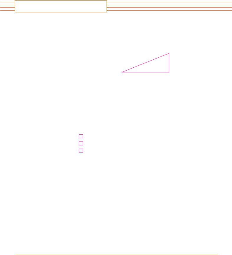
	EXAMPLE 1 Express the hypotenuse h of a right triangle with area 25 m2 as a function of
	its perimeter P.
N Understand the problem	SOLUTION Let’s ﬁrst sort out the information by identifying the unknown quantity and the data:
	Unknown: hypotenuse h
	Given quantities: perimeter P, area 25 m2
N Draw a diagram	It helps to draw a diagram and we do so in Figure 1.
	h
		b

FIGURE 1	a

N N

Connect the given with the unknown Introduce something extra

In order to connect the given quantities to the unknown, we introduce two extra variables a and b, which are the lengths of the other two sides of the triangle. This enables us to express the given condition, which is that the triangle is right-angled, by the Pythagorean Theorem:

h2 ! a2 $ b2

The other connections among the variables come by writing expressions for the area and perimeter:

25 ! 21 ab

P ! a $ b $ h

Since P is given, notice that we now have three equations in the three unknowns a, b, and h:

1	h2	! a2 $ b2
2	25	! 21 ab
3	P	! a $ b $ h

Although we have the correct number of equations, they are not easy to solve in a straightforward fashion. But if we use the problem-solving strategy of trying to recognize some-

N Relate to the familiar thing familiar, then we can solve these equations by an easier method. Look at the right sides of Equations 1, 2, and 3. Do these expressions remind you of anything familiar? Notice that they contain the ingredients of a familiar formula:

$a $ b#2 ! a2 $ 2ab $ b2

Using this idea, we express $a $ b#2 in two ways. From Equations 1 and 2 we have $a $ b#2 ! $a2 $ b2 # $ 2ab ! h2 $ 4$25#

From Equation 3 we have
	$a $ b#2 ! $P ! h#2 ! P2 ! 2Ph $ h2
Thus	h2	$ 100 ! P2 ! 2Ph $ h2
		2Ph ! P2 ! 100
		h !	P2	! 100
		h !		2P
				2P
This is the required expression for h as a function of P.					M

			P R I N C I P L E S O F

		P R O B L E M S O L V I N G


As the next example illustrates, it is often necessary to use the problem-solving prin-
ciple of taking cases when dealing with absolute values.
EXAMPLE 2 Solve the inequality & x ! 3 & $ & x $ 2 & % 11.
SOLUTION Recall the deﬁnition of absolute value:
		x if x # 0
	& x & ! '!x if x % 0
	x ! 3		if x ! 3 # 0
It follows that	& x ! 3 & ! '!$x ! 3#		if x ! 3 % 0
	x ! 3		if x # 3
	! '!x $ 3		if x % 3
	x $ 2		if x $ 2 # 0
Similarly	& x $ 2 & ! '!$x $ 2#		if x $ 2 % 0
	x $ 2		if x # !2
	! '!x ! 2		if x % !2

N Take cases	These expressions show that we must consider three cases:
	x % !2	!2 ( x % 3	x # 3
	CASE I If x % !2, we have
	& x ! 3 & $ & x $ 2 & % 11
		!x $ 3 ! x ! 2 % 11
		!2x % 10
		x ' !5
	CASE II If !2 ( x % 3, the given inequality becomes
	!x $ 3	$ x $ 2 % 11
		5 % 11	(always true)
	CASE III If x # 3, the inequality becomes
		x ! 3 $ x $ 2 % 11
		2x % 12
		x % 6
	Combining cases I, II, and III, we see that the inequality is satisﬁed when !5 % x % 6.
	So the solution is the interval $!5, 6#.		M

P R I N C I P L E S O F

P R O B L E M S O L V I N G

In the following example we ﬁrst guess the answer by looking at special cases and rec-

ognizing a pattern. Then we prove it by mathematical induction.

In using the Principle of Mathematical Induction, we follow three steps:

STEP

Prove that Sn is true when n ! 1.

STEP

Assume that Sn is true when n ! k and deduce that Sn is true when n ! k $ 1.

STEP

Conclude that Sn is true for all n by the Principle of Mathematical Induction.

EXAMPLE 3 If f0$x# ! x"$x $ 1# and fn$1 ! f0 " fn for n ! 0, 1, 2, . . . , ﬁnd a formula

for fn$x#.

N Analogy: Try a similar, simpler problem

SOLUTION We start by ﬁnding formulas for fn$x# for the special cases n ! 1, 2, and 3.

f1$x# ! $ f0 " f0#$x# ! f0$ f0$x## ! f0(

)

x $

x $ 1

2x $ 1

$ 1

x $ 1

f2$x# ! $ f0 " f1 #$x# ! f0$ f1$x## ! f0(2x x$ 1 )

		x				x
!		2x $ 1			!	2x $ 1	!	x
!		x	$	1	!	3x $ 1	!	3x $ 1

	2x $ 1					2x $ 1

f3$x# ! $ f0 " f2 #$x# ! f0$ f2$x## ! f0(3x x$ 1 )

N Look for a pattern

3x $ 1

4x $ 1

3x $ 1

We notice a pattern: The coefﬁcient of x in the denominator of fn$x# is n $ 1 in the three cases we have computed. So we make the guess that, in general,

4	fn$x# !	x
		$n $ 1#x $ 1

To prove this, we use the Principle of Mathematical Induction. We have already veriﬁed that (4) is true for n ! 1. Assume that it is true for n ! k, that is,

fk$x# ! $k $ 1#x $ 1

P R I N C I P L E S O F

P R O B L E M S O L V I N G

Then fk$1$x# ! $ f0 " fk #$x# ! f0$ fk$x## ! f0

($k $ 1#x $ 1 )

$k $ 1# x $ 1

$k $ 2# x $ 1

$k $ 1# x $ 1

This expression shows that (4) is true for n ! k $ 1. Therefore, by mathematical induction, it is true for all positive integers n. M

PROBLEMS

1.One of the legs of a right triangle has length 4 cm. Express the length of the altitude perpendicular to the hypotenuse as a function of the length of the hypotenuse.

2.The altitude perpendicular to the hypotenuse of a right triangle is 12 cm. Express the length of the hypotenuse as a function of the perimeter.

3.Solve the equation & 2x ! 1 & ! & x $ 5 & ! 3.

4.Solve the inequality & x ! 1 & ! & x ! 3 & # 5.

5. Sketch the graph of the function f $x# ! & x2 ! 4& x & $ 3 &.

6.Sketch the graph of the function t$x# ! & x2 ! 1 & ! & x2 ! 4 &.

7.Draw the graph of the equation x $ & x & ! y $ & y &.

8.Draw the graph of the equation x4 ! 4x2 ! x2y2 $ 4y2 ! 0.

9.Sketch the region in the plane consisting of all points $x, y# such that & x & $ & y & ( 1.

10.Sketch the region in the plane consisting of all points $x, y# such that

&x ! y & $ & x & ! & y & ( 2

11.Evaluate $log2 3#$log3 4#$log4 5# &&&$log31 32#.

12.(a) Show that the function f $x# ! ln(x $ sx2 $ 1) is an odd function.

(b)Find the inverse function of f.

13.Solve the inequality ln$x2 ! 2x ! 2# ( 0.

14.Use indirect reasoning to prove that log2 5 is an irrational number.

15.A driver sets out on a journey. For the ﬁrst half of the distance she drives at the leisurely pace of 30 mi"h; she drives the second half at 60 mi"h. What is her average speed on this trip?

16.Is it true that f " $ t $ h# ! f " t $ f " h?

17.Prove that if n is a positive integer, then 7n ! 1 is divisible by 6.

18.Prove that 1 $ 3 $ 5 $ &&& $ $2n ! 1# ! n2.

19.	If f0$x# ! x2		and fn$1$x# ! f0$ fn$x## for n ! 0, 1, 2, . . . , ﬁnd a formula for fn$x#.
20.	(a)	If f0$x# !		1	and fn$1 ! f0 " fn for n ! 0, 1, 2, . . . , ﬁnd an expression for fn$x# and use
				2 ! x

		mathematical induction to prove it.
;	(b)	Graph f0	, f1, f2, f3 on the same screen and describe the effects of repeated composition.

LIMITS AND

DERIVATIVES

The idea of a limit is illustrated by secant lines approaching a tangent line.

In A Preview of Calculus (page 2) we saw how the idea of a limit underlies the various branches of calculus. It is therefore appropriate to begin our study of calculus by investigating limits and their properties. The special type of limit that is used to ﬁnd tangents and velocities gives rise to the central idea in differential calculus, the derivative.

<<< < Предыдущая 1 2 3 4 5 6 7 89 / 919 10 11 12 13 14 15 16 17 18 19 20 21 22 23 24 25 > Следующая >>>

Соседние файлы в предмете [НЕСОРТИРОВАННОЕ]

#
05.02.202055.36 Mб19Calculus, 7th Edition ( PDFDrive.com ).pdf
#
30.12.201945.82 Mб41Complete Solutions Manual for_ SINGLE VARIABLE CALCULUS Early Transcendentals 7th Edition by Stewart ( PDFDrive.com ).pdf
#
30.12.201918.09 Mб36[James_Stewart]_Single_Variable_Calculus_Early_Tr(BookFi).pdf