Добавил:

PavelEngineer Опубликованный материал нарушает ваши авторские права? Сообщите нам.

Вуз:

Севастопольский Государственный Университет

Предмет:

[НЕСОРТИРОВАННОЕ]

Файл:

[James_Stewart]_Single_Variable_Calculus_Early_Tr(BookFi).pdf

Скачиваний:

Добавлен:

30.12.2019

Размер:

18.09 Mб

Скачать

☆

<<< < Предыдущая 11 12 13 14 15 16 17 18 19 20 21 2223 / 9123 24 25 26 27 28 29 30 31 32 33 34 35 > Следующая >>>

SECTION 3.7 RATES OF CHANGE IN THE NATURAL AND SOCIAL SCIENCES |||| 221

3.7

RATES OF CHANGE IN THE NATURAL AND SOCIAL SCIENCES

We know that if y ! f !x", then the derivative dy#dx can be interpreted as the rate of change

of y with respect to x. In this section we examine some of the applications of this idea to

physics, chemistry, biology, economics, and other sciences.

Let’s recall from Section 2.7 the basic idea behind rates of change. If x changes from

x1 to x2, then the change in x is

.x ! x2 # x1

and the corresponding change in y is

.y ! f !x2 " # f !x1"

The difference quotient

f !x2 " # f !x1"

x2 # x1

is the average rate of change of y with respect to x over the interval $x1, x2 % and can be

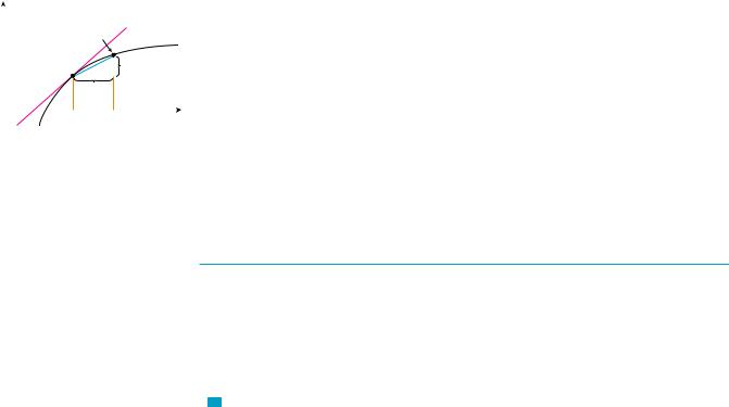
Q{Û,!à}

interpreted as the slope of the secant line PQ in Figure 1. Its limit as .x l 0 is the deriv-

ative f "!x1", which can therefore be interpreted as the instantaneous rate of change of y

P{Ú,!ß}

ëy

with respect to x or the slope of the tangent line at P!x1, f !x1"". Using Leibniz notation,

we write the process in the form

ëx

! lim

mPQ ! average rate of change

.x l0

Whenever the function y ! f !x" has a speciﬁc interpretation in one of the sciences, its

m=f»(Ú)=instantaneous rate

of change

derivative will have a speciﬁc interpretation as a rate of change. (As we discussed in Sec-

FIGURE 1

tion 2.7, the units for dy#dx are the units for y divided by the units for x.) We now look at

some of these interpretations in the natural and social sciences.

PHYSICS

If s ! f !t" is the position function of a particle that is moving in a straight line, then .s#.t represents the average velocity over a time period .t, and v ! ds#dt represents the instantaneous velocity (the rate of change of displacement with respect to time). The instantaneous rate of change of velocity with respect to time is acceleration: a!t" ! v"!t" ! s+!t". This was discussed in Sections 2.7 and 2.8, but now that we know the differentiation formulas, we are able to solve problems involving the motion of objects more easily.

V EXAMPLE 1 The position of a particle is given by the equation s ! f !t" ! t3 # 6t2 ! 9t

where t is measured in seconds and s in meters.

(a)Find the velocity at time t.

(b)What is the velocity after 2 s? After 4 s?

(c)When is the particle at rest?

(d)When is the particle moving forward (that is, in the positive direction)?

(e)Draw a diagram to represent the motion of the particle.

(f)Find the total distance traveled by the particle during the ﬁrst ﬁve seconds.

222|||| CHAPTER 3 DIFFERENTIATION RULES

(g)Find the acceleration at time t and after 4 s.

(h)Graph the position, velocity, and acceleration functions for 0 % t % 5.

(i)When is the particle speeding up? When is it slowing down?

SOLUTION

(a) The velocity function is the derivative of the position function.

s ! f !t" ! t3 ! 6t2 " 9t

v!t" ! dsdt ! 3t2 ! 12t " 9

(b) The velocity after 2 s means the instantaneous velocity when t ! 2, that is,

v!2" ! ds % ! 3!2"2 ! 12!2" " 9 ! !3 m#s dt t!2

The velocity after 4 s is

v!4" ! 3!4"2 ! 12!4" " 9 ! 9 m#s

				3t2 ! 12t " 9 ! 3!t2 ! 4t " 3" ! 3!t ! 1"!t ! 3" ! 0
			and this is true when t ! 1 or t ! 3. Thus the particle is at rest after 1 s and after 3 s.
			(d)	The particle moves in the positive direction when v!t" $ 0, that is,
				3t2 ! 12t " 9 ! 3!t ! 1"!t ! 3" $ 0
			This inequality is true when both factors are positive !t $ 3" or when both factors are
			negative !t # 1". Thus the particle moves in the positive direction in the time intervals
			t # 1 and t $ 3. It moves backward (in the negative direction) when 1 # t # 3.
t=3			(e)	Using the information from part (d) we make a schematic sketch in Figure 2 of the
s=0			motion of the particle back and forth along a line (the s-axis).
			(f)	Because of what we learned in parts (d) and (e), we need to calculate the distances
			traveled during the time intervals [0, 1], [1, 3], and [3, 5] separately.
				The distance traveled in the ﬁrst second is
t=0	t=1	s		The distance traveled in the ﬁrst second is
t=0	t=1	s		$ f !1" ! f !0" $ ! $ 4 ! 0	$ ! 4 m
s=0	s=4			$ f !1" ! f !0" $ ! $ 4 ! 0	$ ! 4 m
FIGURE 2			From t ! 1 to t ! 3 the distance traveled is
			From t ! 1 to t ! 3 the distance traveled is
				$ f !3" ! f !1" $ ! $ 0 ! 4	$ ! 4 m
			From t ! 3 to t ! 5 the distance traveled is
				$ f !5" ! f !3" $ ! $ 20 ! 0	$ ! 20 m

The total distance is 4 " 4 " 20 ! 28 m.

(g) The acceleration is the derivative of the velocity function:

a!t" !	d 2s	!	dv	! 6t ! 12
	dt2		dt

a!4" ! 6!4" ! 12 ! 12 m#s2

SECTION 3.7 RATES OF CHANGE IN THE NATURAL AND SOCIAL SCIENCES |||| 223

(h)

Figure 3 shows the graphs of s, v, and a.

(i)

The particle speeds up when the velocity is positive and increasing (v and a are both

√

positive) and also when the velocity is negative and decreasing (v and a are both nega-

tive). In other words, the particle speeds up when the velocity and acceleration have the

same sign. (The particle is pushed in the same direction it is moving.) From Figure 3 we

see that this happens when 1 # t # 2 and when t $ 3. The particle slows down when

-12

v and a have opposite signs, that is, when 0 % t # 1 and when 2 # t # 3. Figure 4 sum-

marizes the motion of the particle.

FIGURE 3

TEC In Module 3.7 you can see an animation of Figure 4 with an expression for s that you can choose yourself.

FIGURE 4

√

0	1			t
_5	1
_5
forward	backward		forward
slows	speeds	slows	speeds
down	up	down	up	M

EXAMPLE 2 If a rod or piece of wire is homogeneous, then its linear density is uniform and is deﬁned as the mass per unit length !& ! m#l" and measured in kilograms per meter. Suppose, however, that the rod is not homogeneous but that its mass measured from its left end to a point x is m ! f !x", as shown in Figure 5.


FIGURE 5		This part of the rod has mass Ä.		xÁ	xª

	The mass of the part of the rod that lies between x ! x1 and x ! x2 is given by
	'm ! f !x2 " ! f !x1", so the average density of that part of the rod is
		average density !	'm	!	f !x2 " ! f !x1"
			'x		x2 ! x1

If we now let 'x l 0 (that is, x2 l x1), we are computing the average density over smaller and smaller intervals. The linear density & at x1 is the limit of these average densities as 'x l 0; that is, the linear density is the rate of change of mass with respect to length. Symbolically,

! lim	'm	! dm
	'x
'x l0		dx

Thus the linear density of the rod is the derivative of mass with respect to length.

224 |||| CHAPTER 3 DIFFERENTIATION RULES

!	! !	!	!
	! !	!	!

FIGURE 6

For instance, if m ! f !x" ! sx , where x is measured in meters and m in kilograms, then the average density of the part of the rod given by 1 % x % 1.2 is

f !1.2" ! f !1"

! 1

1.2

( 0.48 kg#m

1.2 ! 1

0.2

while the density right at x ! 1 is

! dmdx %x!1

%x!1

! 0.50 kg#m

V EXAMPLE 3 A current exists whenever electric charges move. Figure 6 shows part of a wire and electrons moving through a shaded plane surface. If 'Q is the net charge that passes through this surface during a time period 't, then the average current during this time interval is deﬁned as

average current ! 'Q ! Q2 ! Q1

't t2 ! t1

If we take the limit of this average current over smaller and smaller time intervals, we get what is called the current I at a given time t1:

I ! lim	'Q	! dQ
	't
't l0		dt
Thus the current is the rate at which charge ﬂows through a surface. It is measured in
units of charge per unit time (often coulombs per second, called amperes).			M

Velocity, density, and current are not the only rates of change that are important in physics. Others include power (the rate at which work is done), the rate of heat ﬂow, temperature gradient (the rate of change of temperature with respect to position), and the rate of decay of a radioactive substance in nuclear physics.

CHEMISTRY

EXAMPLE 4 A chemical reaction results in the formation of one or more substances (called products) from one or more starting materials (called reactants). For instance, the “equation”

2H2 " O2 l 2H2O

indicates that two molecules of hydrogen and one molecule of oxygen form two molecules of water. Let’s consider the reaction

A " B l C

where A and B are the reactants and C is the product. The concentration of a reactant A is the number of moles (1 mole ! 6.022 ( 1023 molecules) per liter and is denoted by &A'. The concentration varies during a reaction, so &A', &B', and &C' are all functions of

t2 ! t1

SECTION 3.7 RATES OF CHANGE IN THE NATURAL AND SOCIAL SCIENCES |||| 225

time !t". The average rate of reaction of the product C over a time interval t1 % t % t2 is

'&C' ! &C'!t2 " ! &C'!t1"

But chemists are more interested in the instantaneous rate of reaction, which is obtained by taking the limit of the average rate of reaction as the time interval 't approaches 0:

rate of reaction ! lim	'&C'	!	d&C'
	't		dt
't l0

Since the concentration of the product increases as the reaction proceeds, the derivative d&C'#dt will be positive, and so the rate of reaction of C is positive. The concentrations of the reactants, however, decrease during the reaction, so, to make the rates of reaction of A and B positive numbers, we put minus signs in front of the derivatives d&A'#dt and d&B'#dt. Since &A' and &B' each decrease at the same rate that &C' increases, we have

rate of reaction !

d&C'

! !

d&A'

! !

d&B'

More generally, it turns out that for a reaction of the form

aA " bB l cC " dD

we have

1 d&A'

! !

1 d&B'

1 d&C'

1 d&D'

The rate of reaction can be determined from data and graphical methods. In some cases there are explicit formulas for the concentrations as functions of time, which enable us to compute the rate of reaction (see Exercise 22). M

EXAMPLE 5 One of the quantities of interest in thermodynamics is compressibility. If a given substance is kept at a constant temperature, then its volume V depends on its pressure P. We can consider the rate of change of volume with respect to pressure—namely, the derivative dV#dP. As P increases, V decreases, so dV#dP # 0. The compressibility is deﬁned by introducing a minus sign and dividing this derivative by the volume V:

isothermal compressibility !

1 dV ! ! V dP

Thus * measures how fast, per unit volume, the volume of a substance decreases as the pressure on it increases at constant temperature.

For instance, the volume V (in cubic meters) of a sample of air at 25)C was found to be related to the pressure P (in kilopascals) by the equation

V ! 5P.3

226 |||| CHAPTER 3 DIFFERENTIATION RULES

The rate of change of V with respect to P when P ! 50 kPa is

dPdV %P!50

! !

5.3

%P!50

! !

5.3

! !0.00212 m3#kPa

2500

The compressibility at that pressure is

1 dV

0.00212

* ! !

dP %P!50

! 0.02 !m3#kPa"#m3

5.3

BIOLOGY

EXAMPLE 6 Let n ! f !t" be the number of individuals in an animal or plant population at time t. The change in the population size between the times t ! t1 and t ! t2 is 'n ! f !t2 " ! f !t1", and so the average rate of growth during the time period t1 % t % t2 is

average rate of growth ! 'n ! f !t2 " ! f !t1"

't t2 ! t1

The instantaneous rate of growth is obtained from this average rate of growth by letting the time period 't approach 0:

growth rate ! lim	'n	! dn
	't
't l0		dt

FIGURE 7

A smooth curve approximating a growth function

Strictly speaking, this is not quite accurate because the actual graph of a population function n ! f !t" would be a step function that is discontinuous whenever a birth or death occurs and therefore not differentiable. However, for a large animal or plant population, we can replace the graph by a smooth approximating curve as in Figure 7.

n
0	t

SECTION 3.7 RATES OF CHANGE IN THE NATURAL AND SOCIAL SCIENCES |||| 227

To be more speciﬁc, consider a population of bacteria in a homogeneous nutrient medium. Suppose that by sampling the population at certain intervals it is determined that the population doubles every hour. If the initial population is n0 and the time t is measured in hours, then

f !1" ! 2f !0" ! 2n0 f !2" ! 2f !1" ! 22n0 f !3" ! 2f !2" ! 23n0

and, in general,

f !t" ! 2tn0

The population function is n ! n0 2t. In Section 3.4 we showed that

dxd !ax " ! ax ln a

So the rate of growth of the bacteria population at time t is

dn	!	d	!n02t " ! n02t ln 2
dt		dt

For example, suppose that we start with an initial population of n0 ! 100 bacteria. Then the rate of growth after 4 hours is

dn	! 100 ! 24 ln 2 ! 1600 ln 2	( 1109
dt %t!4	! 100 ! 24 ln 2 ! 1600 ln 2	( 1109
dt %t!4
This means that, after 4 hours, the bacteria population is growing at a rate of about
1109 bacteria per hour.		M

EXAMPLE 7 When we consider the ﬂow of blood through a blood vessel, such as a vein or artery, we can model the shape of the blood vessel by a cylindrical tube with radius R and length l as illustrated in Figure 8.

R r

FIGURE 8

Blood ﬂow in an artery				l

N For more detailed information, see W. Nichols and M. O’Rourke (eds.), McDonald’s Blood Flow in Arteries: Theoretic, Experimental, and Clinical Principles, 4th ed. (New York: Oxford University Press, 1998).

Because of friction at the walls of the tube, the velocity v of the blood is greatest along the central axis of the tube and decreases as the distance r from the axis increases until v becomes 0 at the wall. The relationship between v and r is given by the law of laminar ﬂow discovered by the French physician Jean-Louis-Marie Poiseuille in 1840. This law states that

1	v !	P	!R2 ! r2 "
		4+l

where + is the viscosity of the blood and P is the pressure difference between the ends of the tube. If P and l are constant, then v is a function of r with domain &0, R'.

r2 ! r1

228 |||| CHAPTER 3 DIFFERENTIATION RULES

The average rate of change of the velocity as we move from r ! r1 outward to r ! r2 is given by

''vr ! v!r2 " ! v!r1"

and if we let 'r l 0, we obtain the velocity gradient, that is, the instantaneous rate of change of velocity with respect to r:

velocity gradient ! lim					'v		!	dv

				'r l0	'r dr
Using Equation 1, we obtain
	dv	!	P	!0 ! 2r" ! !			Pr
	dr		4+l			2+l

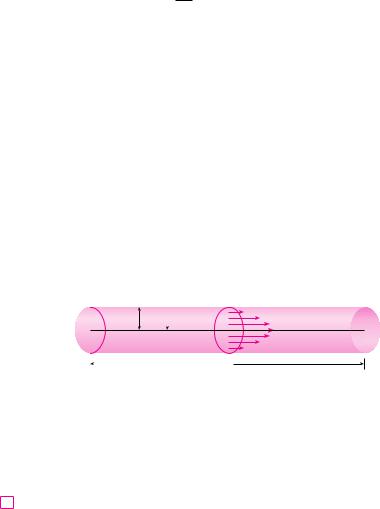
For one of the smaller human arteries we can take + ! 0.027, R ! 0.008 cm, l ! 2 cm, and P ! 4000 dynes#cm2, which gives

		v !		4000	!0.000064		! r2 "
			4!0.027"2

( 1.85 ( 104!6.4 ( 10							!5 ! r2 "
At r ! 0.002 cm the blood is ﬂowing at a speed of
v!0.002" ( 1.85 ( 104!64 ( 10!6 ! 4 ( 10!6 "
		! 1.11 cm#s
and the velocity gradient at that point is
	dv			4000!0.002"
		%r!0.002 !		! 2!0.027"2		( !74		!cm#s"#cm
	dr

To get a feeling for what this statement means, let’s change our units from centimeters to micrometers (1 cm ! 10,000 ,m). Then the radius of the artery is 80 ,m. The velocity at the central axis is 11,850 ,m#s, which decreases to 11,110 ,m#s at a distance of r ! 20 ,m. The fact that dv#dr ! !74 (,m#s)#,m means that, when r ! 20 ,m, the velocity is decreasing at a rate of about 74 ,m#s for each micrometer that we proceed away from the center. M

ECONOMICS

V EXAMPLE 8 Suppose C!x" is the total cost that a company incurs in producing x units of a certain commodity. The function C is called a cost function. If the number of items produced is increased from x1 to x2, then the additional cost is 'C ! C!x2 " ! C!x1", and the average rate of change of the cost is

'C		C!x2 " ! C!x1	"		C!x1 " 'x" ! C!x1"
	!			!
'x	!	x2 ! x1		!	'x

The limit of this quantity as 'x l 0, that is, the instantaneous rate of change of cost

SECTION 3.7 RATES OF CHANGE IN THE NATURAL AND SOCIAL SCIENCES |||| 229

with respect to the number of items produced, is called the marginal cost by economists:

marginal cost ! lim	'C	! dC
	'x
'x l0		dx

[Since x often takes on only integer values, it may not make literal sense to let 'x approach 0, but we can always replace C!x" by a smooth approximating function as in Example 6.]

Taking 'x ! 1 and n large (so that 'x is small compared to n), we have

C-!n" ( C!n " 1" ! C!n"

Thus the marginal cost of producing n units is approximately equal to the cost of producing one more unit [the !n " 1"st unit].

It is often appropriate to represent a total cost function by a polynomial

C!x" ! a " bx " cx2 " dx3

where a represents the overhead cost (rent, heat, maintenance) and the other terms represent the cost of raw materials, labor, and so on. (The cost of raw materials may be proportional to x, but labor costs might depend partly on higher powers of x because of overtime costs and inefﬁciencies involved in large-scale operations.)

For instance, suppose a company has estimated that the cost (in dollars) of producing x items is

C!x" ! 10,000 " 5x " 0.01x2

Then the marginal cost function is

C-!x" ! 5 " 0.02x

The marginal cost at the production level of 500 items is

C-!500" ! 5 " 0.02!500" ! $15#item

This gives the rate at which costs are increasing with respect to the production level when x ! 500 and predicts the cost of the 501st item.

The actual cost of producing the 501st item is

C!501" ! C!500" ! &10,000 " 5!501" " 0.01!501"2 '

!! &10,000 " 5!500" " 0.01!500"2 '

!$15.01

Notice that C-!500" ( C!501" ! C!500".

Economists also study marginal demand, marginal revenue, and marginal proﬁt, which are the derivatives of the demand, revenue, and proﬁt functions. These will be considered in Chapter 4 after we have developed techniques for ﬁnding the maximum and minimum values of functions.

OTHER SCIENCES

Rates of change occur in all the sciences. A geologist is interested in knowing the rate at which an intruded body of molten rock cools by conduction of heat into surrounding rocks. An engineer wants to know the rate at which water ﬂows into or out of a reservoir. An

230 |||| CHAPTER 3 DIFFERENTIATION RULES

urban geographer is interested in the rate of change of the population density in a city as the distance from the city center increases. A meteorologist is concerned with the rate of change of atmospheric pressure with respect to height (see Exercise 17 in Section 3.8).

In psychology, those interested in learning theory study the so-called learning curve, which graphs the performance P!t" of someone learning a skill as a function of the training time t. Of particular interest is the rate at which performance improves as time passes, that is, dP#dt.

In sociology, differential calculus is used in analyzing the spread of rumors (or innovations or fads or fashions). If p!t" denotes the proportion of a population that knows a rumor by time t, then the derivative dp#dt represents the rate of spread of the rumor (see Exercise 82 in Section 3.4).

A SINGLE IDEA, MANY INTERPRETATIONS

Velocity, density, current, power, and temperature gradient in physics; rate of reaction and compressibility in chemistry; rate of growth and blood velocity gradient in biology; marginal cost and marginal proﬁt in economics; rate of heat ﬂow in geology; rate of improvement of performance in psychology; rate of spread of a rumor in sociology—these are all special cases of a single mathematical concept, the derivative.

This is an illustration of the fact that part of the power of mathematics lies in its abstractness. A single abstract mathematical concept (such as the derivative) can have different interpretations in each of the sciences. When we develop the properties of the mathematical concept once and for all, we can then turn around and apply these results to all of the sciences. This is much more efﬁcient than developing properties of special concepts in each separate science. The French mathematician Joseph Fourier (1768–1830) put it succinctly: “Mathematics compares the most diverse phenomena and discovers the secret analogies that unite them.”

3.7

1– 4 t .

(a)

(b)

(c)

(d)

(e)

(f)

(g) ; (h)

(i)

EXERCISES

A particle moves according to a law of motion s ! f !t",

(a)

√

(b)

√

0, where t is measured in seconds and s in feet.

Find the velocity at time t.

What is the velocity after 3 s?

When is the particle at rest?

When is the particle moving in the positive direction?

Find the total distance traveled during the ﬁrst 8 s.

Draw a diagram like Figure 2 to illustrate the motion of the

Graphs of the position functions of two particles are shown,

particle.

where t is measured in seconds. When is each particle speed-

Find the acceleration at time t and after 3 s.

ing up? When is it slowing down? Explain.

Graph the position, velocity, and acceleration functions for

(a)

(b)

0 % t % 8.

When is the particle speeding up? When is it slowing down?

f !t" ! t3 ! 12t2 " 36t

2. f !t" ! 0.01t4 ! 0.04t3

f !t" ! cos!/t#4", t % 10

4. f !t" ! te!t#2

Graphs of the velocity functions of two particles are shown,

The position function of a particle is given by

where t is measured in seconds. When is each particle speed-

s ! t3 ! 4.5t2 ! 7t, t . 0.

ing up? When is it slowing down? Explain.

(a) When does the particle reach a velocity of 5 m#s?

SECTION 3.7 RATES OF CHANGE IN THE NATURAL AND SOCIAL SCIENCES |||| 231

(b)When is the acceleration 0? What is the signiﬁcance of this value of t ?

8.If a ball is given a push so that it has an initial velocity of

5 m#s down a certain inclined plane, then the distance it has rolled after t seconds is s ! 5t " 3t2.

(a)Find the velocity after 2 s.

(b)How long does it take for the velocity to reach 35 m#s?

9.If a stone is thrown vertically upward from the surface of the moon with a velocity of 10 m#s, its height (in meters) after t seconds is h ! 10t ! 0.83t2.

(a)What is the velocity of the stone after 3 s?

(b)What is the velocity of the stone after it has risen 25 m?

10.If a ball is thrown vertically upward with a velocity of 80 ft#s, then its height after t seconds is s ! 80t ! 16t2.

(a)What is the maximum height reached by the ball?

(b)What is the velocity of the ball when it is 96 ft above the ground on its way up? On its way down?

11.(a) A company makes computer chips from square wafers

of silicon. It wants to keep the side length of a wafer very close to 15 mm and it wants to know how the area A!x" of a wafer changes when the side length x changes. Find A-!15" and explain its meaning in this situation.

(b)Show that the rate of change of the area of a square with respect to its side length is half its perimeter. Try to explain geometrically why this is true by drawing a square whose side length x is increased by an amount 'x. How can you approximate the resulting change in area 'A if 'x is small?

12.(a) Sodium chlorate crystals are easy to grow in the shape of cubes by allowing a solution of water and sodium chlorate to evaporate slowly. If V is the volume of such a cube with side length x, calculate dV#dx when x ! 3 mm and explain its meaning.

(b)Show that the rate of change of the volume of a cube with respect to its edge length is equal to half the surface area of the cube. Explain geometrically why this result is true by arguing by analogy with Exercise 11(b).

13.(a) Find the average rate of change of the area of a circle with respect to its radius r as r changes from

(i) 2 to 3

(ii) 2 to 2.5

(iii) 2 to 2.1

(b)Find the instantaneous rate of change when r ! 2.

(c)Show that the rate of change of the area of a circle with respect to its radius (at any r) is equal to the circumference of the circle. Try to explain geometrically why this is true by drawing a circle whose radius is increased

by an amount 'r. How can you approximate the resulting change in area 'A if 'r is small?

14.A stone is dropped into a lake, creating a circular ripple that travels outward at a speed of 60 cm#s. Find the rate at which the area within the circle is increasing after (a) 1 s, (b) 3 s, and (c) 5 s. What can you conclude?

15.A spherical balloon is being inﬂated. Find the rate of increase of the surface area !S ! 4/r2 " with respect to the radius r when r is (a) 1 ft, (b) 2 ft, and (c) 3 ft. What conclusion can you make?

16.(a) The volume of a growing spherical cell is V ! 43 /r3, where the radius r is measured in micrometers

(1 ,m ! 10!6 m). Find the average rate of change of V with respect to r when r changes from

(i) 5 to 8 ,m (ii) 5 to 6 ,m (iii) 5 to 5.1 ,m

(b) Find the instantaneous rate of change of V with respect to r when r ! 5 ,m.

(c) Show that the rate of change of the volume of a sphere with respect to its radius is equal to its surface area. Explain geometrically why this result is true. Argue by analogy with Exercise 13(c).

17. The mass of the part of a metal rod that lies between its left end and a point x meters to the right is 3x2 kg. Find the linear density (see Example 2) when x is (a) 1 m, (b) 2 m, and

18. If a tank holds 5000 gallons of water, which drains from the bottom of the tank in 40 minutes, then Torricelli’s Law gives

the volume V of water remaining in the tank after t minutes as
V ! 5000)1 ! 40t *2	0 % t % 40

Find the rate at which water is draining from the tank after

(a)5 min, (b) 10 min, (c) 20 min, and (d) 40 min. At what time is the water ﬂowing out the fastest? The slowest? Summarize your ﬁndings.

19.The quantity of charge Q in coulombs (C) that has passed through a point in a wire up to time t (measured in seconds) is given by Q!t" ! t3 ! 2t2 " 6t " 2. Find the current when

(a)t ! 0.5 s and (b) t ! 1 s. [See Example 3. The unit of current is an ampere (1 A ! 1 C#s).] At what time is the current lowest?

20.Newton’s Law of Gravitation says that the magnitude F of the force exerted by a body of mass m on a body of mass M is

GmM F ! r2

where G is the gravitational constant and r is the distance between the bodies.

(a)Find dF#dr and explain its meaning. What does the minus sign indicate?

(b)Suppose it is known that the earth attracts an object with a force that decreases at the rate of 2 N#km when

r ! 20,000 km. How fast does this force change when r ! 10,000 km?

21.Boyle’s Law states that when a sample of gas is compressed at a constant temperature, the product of the pressure and the volume remains constant: PV ! C.

(a)Find the rate of change of volume with respect to

pressure.

232|||| CHAPTER 3 DIFFERENTIATION RULES

(b)A sample of gas is in a container at low pressure and is steadily compressed at constant temperature for 10 minutes. Is the volume decreasing more rapidly at the beginning or the end of the 10 minutes? Explain.

(c)Prove that the isothermal compressibility (see

Example 5) is given by ' ! 1"P.

22.If, in Example 4, one molecule of the product C is formed from one molecule of the reactant A and one molecule of the reactant B, and the initial concentrations of A and B have a common value &A% ! &B% ! a moles"L, then

&C% ! a2kt"#akt $ 1$ where k is a constant.

(a)Find the rate of reaction at time t.

(b)Show that if x ! &C%, then

dxdt ! k#a % x$2

(c)What happens to the concentration as t l &?

(d)What happens to the rate of reaction as t l &?

(e)What do the results of parts (c) and (d) mean in practical terms?

23.In Example 6 we considered a bacteria population that doubles every hour. Suppose that another population of bacteria triples every hour and starts with 400 bacteria. Find an expression for the number n of bacteria after t hours and use it to estimate the rate of growth of the bacteria population after 2.5 hours.

24.The number of yeast cells in a laboratory culture increases rapidly initially but levels off eventually. The population is modeled by the function

n ! f # t$ ! 1 $ be%0.7t

where t is measured in hours. At time t ! 0 the population is 20 cells and is increasing at a rate of 12 cells" hour. Find the values of a and b. According to this model, what happens to the yeast population in the long run?

;25. The table gives the population of the world in the 20th century.

	Population		Population
Year	(in millions)	Year	(in millions)

1900	1650	1960	3040
1910	1750	1970	3710
1920	1860	1980	4450
1930	2070	1990	5280
1940	2300	2000	6080
1950	2560

(a)Estimate the rate of population growth in 1920 and in 1980 by averaging the slopes of two secant lines.

(b)Use a graphing calculator or computer to ﬁnd a cubic

function (a third-degree polynomial) that models the data.

(c)Use your model in part (b) to ﬁnd a model for the rate of population growth in the 20th century.

(d)Use part (c) to estimate the rates of growth in 1920 and 1980. Compare with your estimates in part (a).

(e)Estimate the rate of growth in 1985.

;26. The table shows how the average age of ﬁrst marriage of Japanese women varied in the last half of the 20th century.

t	A#t$	t	A#t$

1950	23.0	1980	25.2
1955	23.8	1985	25.5
1960	24.4	1990	25.9
1965	24.5	1995	26.3
1970	24.2	2000	27.0
1975	24.7

(a)Use a graphing calculator or computer to model these data with a fourth-degree polynomial.

(b)Use part (a) to ﬁnd a model for A##t$.

(c)Estimate the rate of change of marriage age for women in 1990.

(d)Graph the data points and the models for A and A#.

27.Refer to the law of laminar ﬂow given in Example 7. Consider a blood vessel with radius 0.01 cm, length 3 cm,

pressure difference 3000 dynes"cm2, and viscosity " ! 0.027.

(a)Find the velocity of the blood along the centerline r ! 0, at radius r ! 0.005 cm, and at the wall r ! R ! 0.01 cm.

(b)Find the velocity gradient at r ! 0, r ! 0.005, and r ! 0.01.

(c)Where is the velocity the greatest? Where is the velocity changing most?

28.The frequency of vibrations of a vibrating violin string is given by

!Tf ! 1

where L is the length of the string, T is its tension, and ! is its linear density. [See Chapter 11 in D. E. Hall, Musical Acoustics, 3d ed. (Paciﬁc Grove, CA: Brooks/Cole, 2002).]

(a) Find the rate of change of the frequency with respect to

(i)	the length (when T and ! are constant),
(ii)	the tension (when L and ! are constant), and

(iii)the linear density (when L and T are constant).

(b)The pitch of a note (how high or low the note sounds) is determined by the frequency f. (The higher the frequency, the higher the pitch.) Use the signs of the derivatives in part (a) to determine what happens to the pitch of a note

(i)when the effective length of a string is decreased by placing a ﬁnger on the string so a shorter portion of

the string vibrates,

(ii)when the tension is increased by turning a tuning peg,

(iii)when the linear density is increased by switching to another string.

<<< < Предыдущая 11 12 13 14 15 16 17 18 19 20 21 2223 / 9123 24 25 26 27 28 29 30 31 32 33 34 35 > Следующая >>>

Соседние файлы в предмете [НЕСОРТИРОВАННОЕ]

#
05.02.202055.36 Mб19Calculus, 7th Edition ( PDFDrive.com ).pdf
#
30.12.201945.82 Mб41Complete Solutions Manual for_ SINGLE VARIABLE CALCULUS Early Transcendentals 7th Edition by Stewart ( PDFDrive.com ).pdf
#
30.12.201918.09 Mб36[James_Stewart]_Single_Variable_Calculus_Early_Tr(BookFi).pdf