

- •CONTENTS
- •Preface
- •To the Student
- •Diagnostic Tests
- •1.1 Four Ways to Represent a Function
- •1.2 Mathematical Models: A Catalog of Essential Functions
- •1.3 New Functions from Old Functions
- •1.4 Graphing Calculators and Computers
- •1.6 Inverse Functions and Logarithms
- •Review
- •2.1 The Tangent and Velocity Problems
- •2.2 The Limit of a Function
- •2.3 Calculating Limits Using the Limit Laws
- •2.4 The Precise Definition of a Limit
- •2.5 Continuity
- •2.6 Limits at Infinity; Horizontal Asymptotes
- •2.7 Derivatives and Rates of Change
- •Review
- •3.2 The Product and Quotient Rules
- •3.3 Derivatives of Trigonometric Functions
- •3.4 The Chain Rule
- •3.5 Implicit Differentiation
- •3.6 Derivatives of Logarithmic Functions
- •3.7 Rates of Change in the Natural and Social Sciences
- •3.8 Exponential Growth and Decay
- •3.9 Related Rates
- •3.10 Linear Approximations and Differentials
- •3.11 Hyperbolic Functions
- •Review
- •4.1 Maximum and Minimum Values
- •4.2 The Mean Value Theorem
- •4.3 How Derivatives Affect the Shape of a Graph
- •4.5 Summary of Curve Sketching
- •4.7 Optimization Problems
- •Review
- •5 INTEGRALS
- •5.1 Areas and Distances
- •5.2 The Definite Integral
- •5.3 The Fundamental Theorem of Calculus
- •5.4 Indefinite Integrals and the Net Change Theorem
- •5.5 The Substitution Rule
- •6.1 Areas between Curves
- •6.2 Volumes
- •6.3 Volumes by Cylindrical Shells
- •6.4 Work
- •6.5 Average Value of a Function
- •Review
- •7.1 Integration by Parts
- •7.2 Trigonometric Integrals
- •7.3 Trigonometric Substitution
- •7.4 Integration of Rational Functions by Partial Fractions
- •7.5 Strategy for Integration
- •7.6 Integration Using Tables and Computer Algebra Systems
- •7.7 Approximate Integration
- •7.8 Improper Integrals
- •Review
- •8.1 Arc Length
- •8.2 Area of a Surface of Revolution
- •8.3 Applications to Physics and Engineering
- •8.4 Applications to Economics and Biology
- •8.5 Probability
- •Review
- •9.1 Modeling with Differential Equations
- •9.2 Direction Fields and Euler’s Method
- •9.3 Separable Equations
- •9.4 Models for Population Growth
- •9.5 Linear Equations
- •9.6 Predator-Prey Systems
- •Review
- •10.1 Curves Defined by Parametric Equations
- •10.2 Calculus with Parametric Curves
- •10.3 Polar Coordinates
- •10.4 Areas and Lengths in Polar Coordinates
- •10.5 Conic Sections
- •10.6 Conic Sections in Polar Coordinates
- •Review
- •11.1 Sequences
- •11.2 Series
- •11.3 The Integral Test and Estimates of Sums
- •11.4 The Comparison Tests
- •11.5 Alternating Series
- •11.6 Absolute Convergence and the Ratio and Root Tests
- •11.7 Strategy for Testing Series
- •11.8 Power Series
- •11.9 Representations of Functions as Power Series
- •11.10 Taylor and Maclaurin Series
- •11.11 Applications of Taylor Polynomials
- •Review
- •APPENDIXES
- •A Numbers, Inequalities, and Absolute Values
- •B Coordinate Geometry and Lines
- •E Sigma Notation
- •F Proofs of Theorems
- •G The Logarithm Defined as an Integral
- •INDEX

SECTION 5.3 THE FUNDAMENTAL THEOREM OF CALCULUS |||| 379
D I S C O V E R Y P R O J E C T
AREA FUNCTIONS
1.(a) Draw the line y ! 2t # 1 and use geometry to find the area under this line, above the t-axis, and between the vertical lines t ! 1 and t ! 3.
(b)If x ) 1, let A! x" be the area of the region that lies under the line y ! 2t # 1 between t ! 1 and t ! x. Sketch this region and use geometry to find an expression for A! x".
(c)Differentiate the area function A! x". What do you notice?
2.(a) If x " %1, let
A! x" ! y%x1 !1 # t2 " dt
A! x" represents the area of a region. Sketch that region.
(b)Use the result of Exercise 28 in Section 5.2 to find an expression for A! x".
(c)Find A+! x". What do you notice?
(d)If x " %1 and h is a small positive number, then A! x # h" % A! x" represents the area of a region. Describe and sketch the region.
(e)Draw a rectangle that approximates the region in part (d). By comparing the areas of these two regions, show that
A! x # h" % A! x" ( 1 # x2 h
(f) Use part (e) to give an intuitive explanation for the result of part (c).
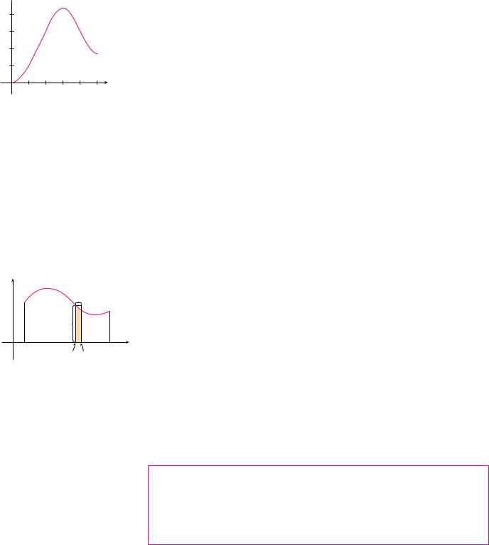
; 3. (a) Draw the graph of the function f ! x" ! cos! x2 " in the viewing rectangle &0, 2' by &%1.25, 1.25'.
(b) If we define a new function t by
t! x" ! y0x cos!t2 " dt
then t! x" is the area under the graph of f from 0 to x [until f ! x" becomes negative, at which point t! x" becomes a difference of areas]. Use part (a) to determine the value of x at which t! x" starts to decrease. [Unlike the integral in Problem 2, it is impossible to evaluate the integral defining t to obtain an explicit expression for t! x".]
(c)Use the integration command on your calculator or computer to estimate t!0.2", t!0.4", t!0.6", . . . , t!1.8", t!2". Then use these values to sketch a graph of t.
(d)Use your graph of t from part (c) to sketch the graph of t+ using the interpretation of t+! x" as the slope of a tangent line. How does the graph of t+ compare with the graph of f ?
4.Suppose f is a continuous function on the interval &a, b' and we define a new function t by the equation
t! x" ! yax f !t" dt
Based on your results in Problems 1–3, conjecture an expression for t+! x".
 5.3 THE FUNDAMENTAL THEOREM OF CALCULUS
The Fundamental Theorem of Calculus is appropriately named because it establishes a connection between the two branches of calculus: differential calculus and integral calculus. Differential calculus arose from the tangent problem, whereas integral calculus arose from a seemingly unrelated problem, the area problem. Newton’s mentor at Cambridge,

380 |||| CHAPTER 5 INTEGRALS
y
y=f(t)
area=©
0 |
a |
x |
b |
t |
FIGURE 1
y |
|
|
|
|
2 |
|
|
y=f(t) |
|
1 |
|
|
|
|
|
|
|
|
|
0 |
1 |
2 |
4 |
t |
FIGURE 2
Isaac Barrow (1630–1677), discovered that these two problems are actually closely related. In fact, he realized that differentiation and integration are inverse processes. The Fundamental Theorem of Calculus gives the precise inverse relationship between the derivative and the integral. It was Newton and Leibniz who exploited this relationship and used it to develop calculus into a systematic mathematical method. In particular, they saw that the Fundamental Theorem enabled them to compute areas and integrals very easily without having to compute them as limits of sums as we did in Sections 5.1 and 5.2.
The first part of the Fundamental Theorem deals with functions defined by an equation of the form
1 t! x" ! yax f !t" dt
where f is a continuous function on &a, b' and x varies between a and b. Observe that t depends only on x, which appears as the variable upper limit in the integral. If x is a fixed
number, then the integral xx f !t" dt is a definite number. If we then let x vary, the number xx ! " a t! "
a f t dt also varies and defines a function of x denoted by x .
If f happens to be a positive function, then t! x" can be interpreted as the area under the graph of f from a to x, where x can vary from a to b. (Think of t as the “area so far” function; see Figure 1.)
V EXAMPLE 1 If f is the function whose graph is shown in Figure 2 and
t! x" ! x0x f !t" dt, find the values of t!0", t!1", t!2", t!3", t!4", and t!5". Then sketch a rough graph of t.
SOLUTION First we notice that t!0" ! x00 f !t" dt ! 0. From Figure 3 we see that t!1" is the area of a triangle:
t!1" ! y01 f !t" dt ! 12 !1 ! 2" ! 1
To find t!2" we add to t!1" the area of a rectangle:
t!2" ! y02 f !t" dt ! y01 f !t" dt # y12 f !t" dt ! 1 # !1 ! 2" ! 3
We estimate that the area under f from 2 to 3 is about 1.3, so
t!3" ! t!2" # y23 f !t" dt ( 3 # 1.3 ! 4.3
y |
|
|
2 |
|
|
1 |
|
|
0 |
1 |
t |
|
g(1)=1 |
|
FIGURE 3
y |
|
|
|
2 |
|
|
|
1 |
|
|
|
0 |
1 |
2 |
t |
|
g(2)=3 |
|
|
y |
|
|
|
|
2 |
|
|
|
|
1 |
|
|
|
|
0 |
1 |
2 |
3 |
t |
|
g(3)•4.3 |
|
|
|
y |
|
|
|
|
2 |
|
|
|
|
1 |
|
|
|
|
0 |
1 |
2 |
4 |
t |
|
|
g(4)•3 |
|
|
y |
|
|
|
|
2 |
|
|
|
|
1 |
|
|
|
|
0 |
1 |
2 |
4 |
t |
|
|
g(5)•1.7 |
|
|
y
4 g
3
2
1
0 |
1 |
2 |
3 |
4 |
5 |
x |
FIGURE 4
©=jax f(t)!dt
y |
|
|
|
|
|
|
h |
|
|
|
Ä |
|
|
|
0 a |
x |
x+h |
b |
t |
|
|
|
FIGURE 5
N We abbreviate the name of this theorem as FTC1. In words, it says that the derivative of a definite integral with respect to its upper limit is the integrand evaluated at the upper limit.
SECTION 5.3 THE FUNDAMENTAL THEOREM OF CALCULUS |||| 381
For t ) 3, f !t" is negative and so we start subtracting areas:
t!4" ! t!3" # y34 f !t" dt ( 4.3 # !%1.3" ! 3.0
t!5" ! t!4" # y45 f !t" dt ( 3 # !%1.3" ! 1.7
We use these values to sketch the graph of t in Figure 4. Notice that, because f !t" is
positive for t ! 3, we keep adding area for t ! 3 and so t is increasing up to x ! 3, |
|
||
where it attains a maximum value. For x ) 3, t decreases because f !t" is negative. |
M |
||
If we take f !t" ! t and a ! 0, then, using Exercise 27 in Section 5.2, we have |
|
||
x |
x2 |
|
|
t! x" ! y0 t dt ! |
|
|
|
2 |
|
|
|
Notice that t+!x" ! x, that is, t+ ! f. In other words, if t is defined as the integral of f by Equation 1, then t turns out to be an antiderivative of f, at least in this case. And if we sketch the derivative of the function t shown in Figure 4 by estimating slopes of tangents, we get a graph like that of f in Figure 2. So we suspect that t+! f in Example 1 too.
To see why this might be generally true we consider any continuous function f with f !x" " 0. Then t! x" ! xax f !t" dt can be interpreted as the area under the graph of f from a to x, as in Figure 1.
In order to compute t+! x" from the definition of derivative we first observe that, for h ) 0, t! x # h" % t! x" is obtained by subtracting areas, so it is the area under the graph of f from x to x # h (the gold area in Figure 5). For small h you can see from the figure that this area is approximately equal to the area of the rectangle with height f ! x" and width h:
t!x # h" % t! x" ( hf ! x"
so |
|
t! x # h" % t!x" |
( f !x" |
|
||
|
|
|
||||
|
|
|
h |
|
|
|
Intuitively, we therefore expect that |
|
|
|
|
||
|
t+!x" ! lim |
t! x # h" % t! x" |
|
! f ! x" |
||
|
|
|||||
|
|
h l0 |
h |
|
|
|
The fact that this is true, even when f is not necessarily positive, is the first part of the Fundamental Theorem of Calculus.
THE FUNDAMENTAL THEOREM OF CALCULUS, PART 1 If f is continuous on &a, b', then the function t defined by
t! x" ! yax f !t" dt a ( x ( b
is continuous on &a, b' and differentiable on !a, b", and t+!x" ! f !x".
382 |||| CHAPTER 5 INTEGRALS
y
y=Ä
M
m
0x u √=x+h x
FIGURE 6
TEC Module 5.3 provides visual evidence for FTC1.
PROOF If x and x # h are in !a, b", then
t! x # h" % t! x" ! yax#h f !t" dt % yax f !t" dt
|
! ,yax f !t" dt # yxx#h f !t" dt- % yax f !t" dt (by Property 5) |
|||||
|
! yxx#h f !t" dt |
|
|
|
|
|
and so, for h " 0, |
|
|
|
|
|
|
|
|
t! x # h" % t! x" |
1 |
x#h |
|
|
2 |
|
|
! |
|
yx |
f !t" dt |
|
h |
h |
||||
For now let us assume that h ) 0. Since f is continuous on &x, x # h', the Extreme Value Theorem says that there are numbers u and v in &x, x # h' such that f !u" ! m and f !v" ! M, where m and M are the absolute minimum and maximum values of f on &x, x # h'. (See Figure 6.)
By Property 8 of integrals, we have
mh ( yxx#h f !t" dt ( Mh
that is, |
x#h |
|
|
f !u"h ( yx |
f !t" dt ( f !v"h |
||
|
Since h ) 0, we can divide this inequality by h:
f !u" ( 1h yxx#h f !t" dt ( f !v"
Now we use Equation 2 to replace the middle part of this inequality:
3 |
f !u" ( |
t! x # h" % t!x" |
( f !v" |
|
h |
||||
|
|
|
Inequality 3 can be proved in a similar manner for the case h ! 0. (See Exercise 67.) Now we let h l 0. Then u l x and v l x, since u and v lie between x and x # h.
Therefore
lim f !u" ! lim f !u" ! f ! x"
|
h l0 |
u lx |
and |
lim f !v" ! lim f !v" ! f ! x" |
|
|
h l0 |
v lx |
because f is continuous at x. We conclude, from (3) and the Squeeze Theorem, that

y 1
1
f
S
01
FIGURE 7
Ä=sin(π≈/2) S(x)=j0x !sin(πt@/2)!dt
y
0.5
1
FIGURE 8
The Fresnel function
S(x)=j0x !sin(πt@/2)!dt
|
|
|
SECTION 5.3 THE FUNDAMENTAL THEOREM OF CALCULUS |||| |
383 |
|||||||||||
|
|
4 |
|
t+! x" ! lim |
|
t! x # h" % t! x" |
! f ! x" |
|
|
|
|||||
|
|
|
|
|
|
|
|
||||||||
|
|
|
|
|
h l0 |
|
|
h |
|
|
|
||||
|
|
If x ! a or b, then Equation 4 can be interpreted as a one-sided limit. Then Theo- |
|
||||||||||||
|
rem 2.8.4 (modified for one-sided limits) shows that t is continuous on &a, b'. |
M |
|||||||||||||
|
|
Using Leibniz notation for derivatives, we can write FTC1 as |
|
|
|
||||||||||
|
|
5 |
|
|
|
d |
|
yax f !t" dt ! f ! x" |
|
|
|
||||
|
|
|
|
|
dx |
|
|
|
|||||||
|
when f |
is continuous. Roughly speaking, Equation 5 says that if we first integrate f |
and |
||||||||||||
|
then differentiate the result, we get back to the original function f. |
|
|
|
|||||||||||
|
|
|
|
|
|
|
|
|
|
|
x |
|
|
|
|
|
|
|
|
|
|
|
|
|
|
|
|
|
|
||
|
V |
EXAMPLE 2 Find the derivative of the function t! x" ! y0 s1 # t |
2 |
dt. |
|
||||||||||
|
|
|
|
||||||||||||
|
|
Since f !t" ! s |
|
is continuous, Part 1 of the Fundamental Theorem of |
|
||||||||||
|
SOLUTION |
1 # t2 |
|
||||||||||||
|
Calculus gives |
|
|
|
|
|
|
|
|
|
|||||
|
|
|
|
|
|
t+! x" ! s |
|
|
|
|
|
|
|
||
|
|
|
1 # x2 |
|
|
M |
|||||||||
|
EXAMPLE 3 Although a formula of the form t!x" ! xax f !t" dt may seem like a strange |
|
|||||||||||||
|
way of defining a function, books on physics, chemistry, and statistics are full of such |
|
|||||||||||||
|
functions. For instance, the Fresnel function |
|
|
|
|||||||||||
x |
|
|
|
|
S! x" ! y0x sin!*t2)2" dt |
|
|
|
|||||||
|
is named after the French physicist Augustin Fresnel (1788–1827), who is famous for his |
||||||||||||||
|
works in optics. This function first appeared in Fresnel’s theory of the diffraction of light |
||||||||||||||
|
waves, but more recently it has been applied to the design of highways. |
|
|||||||||||||
|
|
Part 1 of the Fundamental Theorem tells us how to differentiate the Fresnel function: |
|||||||||||||
|
|
|
|
|
|
S+!x" ! sin!*x2)2" |
|
|
|
||||||
|
This means that we can apply all the methods of differential calculus to analyze S (see |
||||||||||||||
|
Exercise 61). |
|
|
|
|
|
|
|
|
|
|||||
|
|
Figure 7 shows the graphs of f ! x" ! sin!*x2)2" and the Fresnel function |
|
||||||||||||
x |
S! x" ! x0x f !t" dt. A computer was used to graph S by computing the value of this |
|
|||||||||||||
|
integral for many values of x. It does indeed look as if S!x" is the area under the graph |
||||||||||||||
|
of f from 0 to x [until x ( 1.4, when S! x" becomes a difference of areas]. Figure 8 |
|
|||||||||||||
|
shows a larger part of the graph of S. |
|
|
|
|
|
|
|
|
|
|||||
|
|
If we now start with the graph of S in Figure 7 and think about what its derivative |
|
||||||||||||
|
should look like, it seems reasonable that S+!x" ! f !x". [For instance, S is increasing |
|
|||||||||||||
|
when f !x" ) 0 and decreasing when f ! x" ! 0.] So this gives a visual confirmation of |
||||||||||||||
|
Part 1 of the Fundamental Theorem of Calculus. |
|
|
M |
|||||||||||

384 |||| CHAPTER 5 INTEGRALS
EXAMPLE 4 Find dxd y1x 4 sec t dt.
SOLUTION Here we have to be careful to use the Chain Rule in conjunction with FTC1.
Let u ! x4. Then
d |
y1x 4 |
sec t dt ! |
d |
|
y1u sec t dt |
|
|
|||
dx |
dx |
|
|
|
||||||
|
|
! |
|
d |
|
%y1u sec t dt& dudx |
(by the Chain Rule) |
|||
|
|
|
du |
|||||||
|
|
! sec u |
du |
(by FTC1) |
|
|||||
|
|
dx |
|
|
||||||
|
|
! sec!x4 " ! 4x3 |
|
M |
||||||
In Section 5.2 we computed integrals from the definition as a limit of Riemann sums and we saw that this procedure is sometimes long and difficult. The second part of the Fundamental Theorem of Calculus, which follows easily from the first part, provides us with a much simpler method for the evaluation of integrals.
|
THE FUNDAMENTAL THEOREM OF CALCULUS, PART 2 If f is continuous on |
|
|
#a, b$, then |
|
|
b |
f ! x" dx ! F!b" ! F!a" |
N We abbreviate this theorem as FTC2. |
ya |
|
|
|
|
|
where F is any antiderivative of f , that is, a function such that F$ ! f . |
|
|
|
|
P R O O F Let t! x" ! xax f !t" dt. We know from Part 1 that t$! x" ! f ! x"; that is, t is an antiderivative of f. If F is any other antiderivative of f on #a, b$, then we know from Corol-
lary 4.2.7 that F and t differ by a constant:
6 |
F!x" ! t!x" " C |
for a # x # b. But both F and t are continuous on #a, b$ and so, by taking limits of both sides of Equation 6 (as x l a" and x l b!), we see that it also holds when x ! a and x ! b.
If we put x ! a in the formula for t!x", we get |
|
t!a" ! yaa f !t" dt ! 0 |
|
So, using Equation 6 with x ! b and x ! a, we have |
|
F!b" ! F!a" ! # t!b" " C$ ! # t!a" " C$ |
|
! t!b" ! t!a" ! t!b" |
|
! yab f !t" dt |
M |

N Compare the calculation in Example 5 with the much harder one in Example 3 in Section 5.2.
N In applying the Fundamental Theorem we use a particular antiderivative F of f. It is not necessary to use the most general antiderivative.
SECTION 5.3 THE FUNDAMENTAL THEOREM OF CALCULUS |||| 385
Part 2 of the Fundamental Theorem states that if we know an antiderivative F of f, then we can evaluate xb f ! x" dx simply by subtracting the values of F at the endpoints of the interval #a, b$. It’savery surprising that xab f !x" dx, which was defined by a complicated procedure involving all of the values of f ! x" for a % x % b, can be found by knowing the values of F! x" at only two points, a and b.
Although the theorem may be surprising at first glance, it becomes plausible if we interpret it in physical terms. If v!t" is the velocity of an object and s!t" is its position at time t, then v!t" ! s$!t", so s is an antiderivative of v. In Section 5.1 we considered an object that always moves in the positive direction and made the guess that the area under the velocity curve is equal to the distance traveled. In symbols:
yab v!t" dt ! s!b" ! s!a"
That is exactly what FTC2 says in this context.
V EXAMPLE 5 Evaluate the integral y13 ex dx.
SOLUTION The function f ! x" ! ex is continuous everywhere and we know that an antiderivative is F! x" ! ex, so Part 2 of the Fundamental Theorem gives
y13 ex dx ! F!3" ! F!1" ! e3 ! e
Notice that FTC2 says we can use any antiderivative F of f. So we may as well use |
|
||
the simplest one, namely F! x" ! ex, instead of ex " 7 or ex " C. |
M |
||
We often use the notation |
|
|
|
F! x"]ab ! F!b" ! F!a" |
|
|
|
So the equation of FTC2 can be written as |
|
|
|
yab f ! x" dx ! F! x"]ab |
where |
F$! f |
|
Other common notations are F! x" ( ab and #F! x"$ ab.
EXAMPLE 6 Find the area under the parabola y ! x2 from 0 to 1.
SOLUTION An antiderivative of f ! x" ! x2 is F! x" ! 13 x3. The required area A is found using Part 2 of the Fundamental Theorem:
|
|
x3 |
1 |
|
13 |
|
03 |
|
1 |
|
1 |
|
'0 |
|
|
|
|
||||
A ! y0 |
x2 dx ! |
|
! |
|
! |
|
! |
|
M |
|
3 |
3 |
3 |
3 |
If you compare the calculation in Example 6 with the one in Example 2 in Section 5.1, you will see that the Fundamental Theorem gives a much shorter method.
386 |||| CHAPTER 5 INTEGRALS
|
|
|
|
|
|
|
|
EXAMPLE 7 Evaluate y36 |
dx |
. |
|
|
|
|||||||
|
|
|
|
|
|
|
x |
|
|
|
||||||||||
|
|
|
|
|
|
|
|
SOLUTION |
The given integral is an abbreviation for |
|
||||||||||
|
|
|
|
|
|
|
|
|
|
|
|
|
|
|
y36 |
1 |
dx |
|
||
|
|
|
|
|
|
|
|
|
|
|
|
|
|
|
x |
|
||||
|
|
|
|
|
|
|
|
An antiderivative of f ! x" ! 1)x is F!x" ! ln ( x ( and, because 3 % x % 6, we can write |
||||||||||||
|
|
|
|
|
|
|
|
F! x" ! ln x. So |
|
|
|
|
|
|
|
|
|
|
||
|
|
|
|
|
|
|
|
|
|
|
|
|
y36 |
1 |
dx ! ln x]36 ! ln 6 ! ln 3 |
|
||||
|
|
|
|
|
|
|
|
|
|
|
x |
|
||||||||
|
|
|
|
|
|
|
|
|
|
|
6 |
|
|
|
||||||
|
|
|
|
|
|
|
|
|
|
|
|
|
|
|
! ln |
|
|
! ln 2 |
M |
|
|
|
|
|
|
|
|
|
|
|
|
3 |
|||||||||
y |
|
|
|
|
|
|
|
|
|
|
|
|
|
|
|
|
|
|
|
|
|
|
|
|
|
|
|
|
|
|
|
|
|
|
|
|
|
|
|||
1 |
|
|
|
y=cos!x |
|
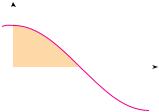
EXAMPLE 8 Find the area under the cosine curve from 0 to b, where 0 % b % |
' |
|||||||||||||
|
|
|
|
|
)2. |
|||||||||||||||
|
|
|
|
area=1 |
|
SOLUTION |
Since an antiderivative of f ! x" ! cos x is F! x" ! sin x, we have |
|
||||||||||||
|
|
|
|
|
|
|
|
|
|
|
|
|
|
|
|
|
|
|||
0 |
|
|
π |
x |
|
|
|
b |
b |
|
||||||||||
|
|
|
|
2 |
|
|
|
A |
! y0 cos x dx ! sin x] |
0 ! sin b ! sin 0 ! sin b |
|
|||||||||
|
|
|
|
|
|
|
|
In particular, taking b ! ')2, we have proved that the area under the cosine curve |
||||||||||||
|
|
|
|
|
|
|
||||||||||||||
FIGURE 9 |
|
|
' |
)2 is sin! |
' |
|
|
|
|
|
|
|
|
M |
||||||
|
|
|
|
|
|
|
|
from 0 to |
)2" ! 1. (See Figure 9.) |
|||||||||||
When the French mathematician Gilles de Roberval first found the area under the sine and cosine curves in 1635, this was a very challenging problem that required a great deal of ingenuity. If we didn’t have the benefit of the Fundamental Theorem, we would have to compute a difficult limit of sums using obscure trigonometric identities (or a computer algebra system as in Exercise 25 in Section 5.1). It was even more difficult for Roberval because the apparatus of limits had not been invented in 1635. But in the 1660s and 1670s, when the Fundamental Theorem was discovered by Barrow and exploited by Newton and Leibniz, such problems became very easy, as you can see from Example 8.
EXAMPLE 9 What is wrong with the following calculation?
|
3 1 |
|
x!1 |
3 |
1 |
|
|
4 |
|
|
|
'!1 ! ! |
|
|
|||||
| |
y!1 |
|
dx ! |
|
|
! 1 |
! ! |
|
|
x2 |
!1 |
3 |
3 |
||||||
SOLUTION To start, we notice that this calculation must be wrong because the answer is negative but f ! x" ! 1)x2 & 0 and Property 6 of integrals says that xab f ! x" dx & 0 when f & 0. The Fundamental Theorem of Calculus applies to continuous functions. It can’t be applied here because f ! x" ! 1)x2 is not continuous on #!1, 3$. In fact, f has an infinite discontinuity at x ! 0, so
y!31 |
1 |
dx |
does not exist |
M |
x2 |

SECTION 5.3 THE FUNDAMENTAL THEOREM OF CALCULUS |||| 387
DIFFERENTIATION AND INTEGRATION AS INVERSE PROCESSES
We end this section by bringing together the two parts of the Fundamental Theorem.
THE FUNDAMENTAL THEOREM OF CALCULUS Suppose f is continuous on #a, b$.
1.If t! x" ! yax f !t" dt, then t$! x" ! f ! x".
2.yab f ! x" dx ! F!b" ! F!a", where F is any antiderivative of f , that is, F$! f .
We noted that Part 1 can be rewritten as
dxd yax f !t" dt ! f ! x"
which says that if f is integrated and then the result is differentiated, we arrive back at the original function f. Since F$! x" ! f ! x", Part 2 can be rewritten as
yab F$! x" dx ! F!b" ! F!a"
This version says that if we take a function F, first differentiate it, and then integrate the result, we arrive back at the original function F, but in the form F!b" ! F!a". Taken together, the two parts of the Fundamental Theorem of Calculus say that differentiation and integration are inverse processes. Each undoes what the other does.
The Fundamental Theorem of Calculus is unquestionably the most important theorem in calculus and, indeed, it ranks as one of the great accomplishments of the human mind. Before it was discovered, from the time of Eudoxus and Archimedes to the time of Galileo and Fermat, problems of finding areas, volumes, and lengths of curves were so difficult that only a genius could meet the challenge. But now, armed with the systematic method that Newton and Leibniz fashioned out of the Fundamental Theorem, we will see in the chapters to come that these challenging problems are accessible to all of us.
5.3EXERCISES
1.Explain exactly what is meant by the statement that “differentiation and integration are inverse processes.”
2.Let t! x" ! x0x f !t" dt, where f is the function whose graph is shown.
y |
|
|
|
|
1 |
|
|
|
|
0 |
1 |
4 |
6 |
t |
(a)Evaluate t! x" for x ! 0, 1, 2, 3, 4, 5, and 6.
(b)Estimate t!7".
(c)Where does t have a maximum value? Where does it have a minimum value?
(d)Sketch a rough graph of t.
3.Let t! x" ! x0x f !t" dt, where f is the function whose graph is shown.
(a)Evaluate t!0", t!1", t!2", t!3", and t!6".
(b)On what interval is t increasing?

388 |||| CHAPTER 5 INTEGRALS
(c)Where does t have a maximum value?
(d)Sketch a rough graph of t.
y |
|
|
|
1 |
|
f |
|
|
|
|
|
0 |
1 |
5 |
t |
4.Let t x xx 3 f t dt, where f is the function whose graph is shown.
(a)Evaluate t 3 and t 3 .
(b)Estimate t 2 , t 1 , and t 0 .
(c)On what interval is t increasing?
(d)Where does t have a maximum value?
(e)Sketch a rough graph of t.
(f)Use the graph in part (e) to sketch the graph of t x . Compare with the graph of f.
y |
|
|
f |
|
|
|
1 |
|
0 |
1 |
t |
5–6 Sketch the area represented by t x . Then find t x in two ways: (a) by using Part 1 of the Fundamental Theorem and (b) by evaluating the integral using Part 2 and then differentiating.
x |
x |
|
|
|
5. t x y1 t 2 dt |
6. t x y0 |
(1 st ) dt |
||
7–18 Use Part 1 of the Fundamental Theorem of Calculus to find the derivative of the function.
|
x |
|
|
|
|
1 |
|
|
|
|
|
|
|
|
x |
2 |
|
|
|
|
|
||
7. |
t x y1 |
|
dt |
8. |
t x y3 |
et |
t dt |
||||||||||||||||
t 3 1 |
|||||||||||||||||||||||
|
y |
|
|
2 |
|
|
|
|
|
|
|
|
|
|
r |
|
|
|
|
|
|
|
|
9. |
t y y2 |
|
t |
sin t dt |
10. |
t r y0 |
sx |
2 |
4 dx |
||||||||||||||
|
|
|
|
|
|
|
|
|
|
|
|
|
|
|
|
|
|
|
|
|
|
|
|
|
|
|
|
|
|
|
|
|
|
|
|
|
|
|
|
|
|
|
|
|
|
||
11. |
F x yx |
|
|
s1 sec t dt |
|
|
|
|
|
|
|
|
|
|
|
||||||||
|
|
|
|
|
|
|
|
|
|
|
|
|
x |
|
|
|
|
|
|
|
|
|
|
|
Hint: yx |
s1 sec t dt y s1 |
sec t dt |
|
|
|
|
|
|||||||||||||||
|
1 |
|
|
|
|
|
|
|
|
|
|
|
|
|
|
|
|
|
|
|
|
||
12. |
G x yx |
|
cos st dt |
|
|
|
|
|
|
|
|
|
|
|
|||||||||
|
1 x |
|
|
|
|
|
|
|
|
|
|
x2 |
|
|
|
|
|
||||||
13. |
h x y2 |
|
|
|
arctan t dt |
14. |
h x y0 |
s1 r 3 dr |
|||||||||||||||
|
|
|
|
|
|
|
|
tan x |
|
|
|
|
|
|
|
|
|
|
|
|
|
|
|
|
|
|
|
cos x |
|
|
|
|
|
||||||||||
15. |
y y0 |
|
|
|
|
st |
st dt |
16. |
y y1 |
|
1 v 2 10 dv |
||||||||||||||||||||||||||||||||
|
|
|
|
|
|
|
1 |
|
|
|
|
|
u 3 |
|
|
|
|
|
|
|
|
|
|
|
0 |
|
|
|
|
|
|
||||||||||||
|
17. |
y y1 3 x |
|
|
|
du |
18. |
y yex |
sin3t dt |
||||||||||||||||||||||||||||||||||
1 u 2 |
|||||||||||||||||||||||||||||||||||||||||||
|
|||||||||||||||||||||||||||||||||||||||||||
|
19– 42 Evaluate the integral. |
|
|
|
|
|
|
|
|
|
|
|
|||||||||||||||||||||||||||||||
19. |
y21 |
x 3 2x dx |
|
|
|
|
|
20. |
y52 6 dx |
|
|
|
|
|
|
||||||||||||||||||||||||||||
|
|
4 |
|
|
|
|
|
|
|
|
|
|
|
|
|
|
|
|
|
|
|
|
|
|
|
|
|
|
|
|
|
1 |
|
|
|
|
|
|
|
|
|
|
|
21. |
y1 |
5 2t 3t 2 dt |
22. |
y0 |
|
(1 21 u 4 52 u9) du |
|||||||||||||||||||||||||||||||||||||
|
|
1 |
|
|
4 5 |
|
|
|
|
|
|
|
|
|
|
|
|
|
|
|
|
|
|
|
|
|
|
8 |
3 |
|
|
|
|
|
|
|
|
||||||
|
|
|
|
|
|
|
|
|
|
|
|
|
|
|
|
|
|
|
|
|
|
|
|
|
|
|
|
|
|
|
|
|
|
||||||||||
23. |
y0 |
x |
|
|
|
|
|
dx |
|
|
|
|
|
|
|
|
|
|
24. |
y1 |
|
sx dx |
|
|
|
|
|
||||||||||||||||
|
|
2 |
3 |
|
|
|
|
|
|
|
|
|
|
|
|
|
|
|
|
|
|
|
|
|
|
|
|
|
|
2 |
|
|
|
|
|
|
|
|
|
||||
|
|
y1 |
|
|
|
|
|
|
|
|
|
|
|
|
|
|
|
|
|
|
|
|
|
|
|
|
|
|
|
|
|
y |
|
|
|
|
|
|
|
|
|||
25. |
|
|
dt |
|
|
|
|
|
|
|
|
|
|
26. |
|
cos d |
|||||||||||||||||||||||||||
t 4 |
|
|
|
|
|
|
|
|
|
|
|
||||||||||||||||||||||||||||||||
|
|
2 |
|
|
|
|
|
|
|
|
|
|
|
|
|
|
|
|
|
|
|
|
|
|
|
|
|
|
|
|
|
1 |
|
|
|
|
|
|
|
|
|
|
|
27. |
y0 |
x 2 x5 dx |
|
|
|
|
|
28. |
y0 |
|
(3 x sx ) dx |
||||||||||||||||||||||||||||||||
|
|
9 |
x 1 |
|
|
|
|
|
|
|
|
|
|
|
|
|
|
|
2 |
|
|
|
|
|
|
|
|
|
|
||||||||||||||
29. |
y1 |
|
|
|
|
|
|
|
|
dx |
|
|
|
|
|
|
|
|
|
|
30. |
y0 |
|
y 1 2y 1 dy |
|||||||||||||||||||
|
|
s |
|
|
|
|
|
|
|
|
|
|
|
|
|
|
|||||||||||||||||||||||||||
|
|
x |
|
|
|
|
|
|
|
|
|
|
|
|
|
||||||||||||||||||||||||||||
|
|
|
|
|
|
|
|
|
|
|
|
|
|
|
|
|
|
|
|
|
|
|
|
|
|
|
|
|
|
|
|
|
|
|
|
|
|
|
|
|
|
||
31. |
y0 4 sec2 t dt |
|
|
|
|
|
|
|
|
|
|
32. |
y0 |
4 sec |
tan d |
||||||||||||||||||||||||||||
|
|
2 |
|
|
|
|
|
|
|
|
|
|
|
|
|
|
|
|
|
|
|
|
|
|
|
|
|
|
|
|
|
1 |
|
|
|
|
|
|
|
|
|
|
|
33. |
y1 |
1 2y 2 dy |
|
|
|
|
|
34. |
y0 |
|
cosh t dt |
||||||||||||||||||||||||||||||||
|
|
9 |
|
1 |
|
|
|
|
|
|
|
|
|
|
|
|
|
|
|
|
|
|
|
|
|
|
|
|
|
|
1 |
|
|
|
|
|
|
|
|
|
|
||
35. |
y1 |
|
|
|
dx |
|
|
|
|
|
|
|
|
|
|
36. |
y0 |
|
10 x dx |
|
|
|
|
|
|||||||||||||||||||
2x |
|
|
|
|
|
|
|
|
|
|
|
|
|
|
|
|
|||||||||||||||||||||||||||
|
|
s3 2 |
|
|
|
|
|
6 |
|
|
|
|
|
|
|
|
|
|
|
|
|
|
|
|
1 |
4 |
|
|
|
|
|
|
|||||||||||
37. |
y1 2 |
|
|
|
|
|
|
|
|
|
|
|
|
dt |
|
|
|
|
|
38. |
y0 |
|
|
|
|
dt |
|||||||||||||||||
|
|
|
s |
|
|
|
|
|
|
|
|
|
|
|
|
t 2 1 |
|||||||||||||||||||||||||||
|
|
|
1 t 2 |
|
|
|
|
|
|
||||||||||||||||||||||||||||||||||
|
|
1 |
|
|
|
|
|
|
|
|
|
|
|
|
|
|
|
|
|
|
|
|
|
|
|
|
|
|
|
|
|
2 4 u2 |
|||||||||||
39. |
y 1 |
eu 1 du |
|
|
|
|
|
|
|
|
|
|
40. |
y1 |
|
|
|
|
|
|
|
du |
|||||||||||||||||||||
|
|
|
|
|
|
|
|
|
|
|
|
u3 |
|
|
|
||||||||||||||||||||||||||||
|
|
|
|
|
|
|
|
|
|
|
|
|
|
|
|
|
|
|
|
|
|
|
|
|
|
|
|
|
|
|
sin x |
if |
0 x 2 |
||||||||||
|
|
f x dx where f x cos x |
|
|
|
|
|
|
|
|
|
|
|
||||||||||||||||||||||||||||||
41. |
y0 |
if 2 x |
|||||||||||||||||||||||||||||||||||||||||
|
|
2 |
|
|
|
|
|
|
|
|
|
|
|
|
|
|
|
|
|
|
|
|
|
|
|
|
2 |
|
if 2 x 0 |
||||||||||||||
42. |
y 2 |
|
f x dx |
|
where f x 4 x 2 |
if 0 x 2 |
|||||||||||||||||||||||||||||||||||||
|
|
|
|
|
|
|
|
|
|
|
|
|
|
|
|
|
|
|
|
|
|
|
|
|
|
|
|
|
|
|
|
|
|
|
|||||||||
; 43– 46 What is wrong with the equation? |
|
|
|
|
|
|
|
|
|
|
|||||||||||||||||||||||||||||||||
|
|
|
|
|
|
|
|
|
|
|
|
|
|
|
|
|
|
x 3 |
1 |
3 |
|
|
|
|
|
|
|
|
|
|
|
|
|||||||||||
|
|
1 |
|
|
|
|
|
|
|
|
|
|
|
|
|
|
|
2 |
|
|
|
|
|
|
|
|
|
|
|
|
|||||||||||||
43. |
y 2 |
x 4 |
|
dx |
|
|
|
|
|
|
|
|
|
|
|
|
|
|
|
|
|
|
|||||||||||||||||||||
|
3 |
8 |
|
|
|
|
|
|
|
|
|
|
|
||||||||||||||||||||||||||||||
|
|
2 |
|
|
4 |
|
|
|
|
|
|
|
|
|
|
|
|
|
|
2 |
2 |
|
3 |
|
|
|
|
|
|
|
|
|
|
|
|
|
|||||||
44. |
|
|
|
|
|
|
dx |
|
|
|
|
|
|
|
|
|
|
|
|
|
|
|
|
|
|
||||||||||||||||||
y 1 x 3 |
|
|
|
|
|
|
|
|
|
|
|
|
|
|
|
|
|
|
|
|
|||||||||||||||||||||||
|
|
|
|
|
|
|
|
|
|
|
|
|
x 2 1 |
2 |
|
|
|
|
|
|
|
|
|
|
|
|
|
||||||||||||||||
|
|
|
|
|
|
|
|
|
|
|
|
|
|
|
|
|
|
|
|
|
|
|
|
|
|
|
|
|
|
|
|
|
|
|
|
|
|
|
|
||||
45. |
y 3 |
|
sec |
tan |
d |
|
sec |
] 3 3 |
|
|
|
|
|
|
|
|
|
|
|
||||||||||||||||||||||||
|
|
|
|
|
|
|
2 |
|
|
|
|
|
|
|
|
|
|
|
|
|
|
|
|
|
|
|
|
|
|
|
|
|
|
|
|
||||||||
|
|
y0 |
|
|
|
|
|
|
|
|
|
|
|
|
|
|
|
|
|
|
|
|
0 |
|
|
|
|
|
|
|
|
|
|
|
|
|
|
||||||
46. |
sec x dx tan x]0 |
|
|
|
|
|
|
|
|
|
|
|
|
|
|
||||||||||||||||||||||||||||
|
|
|
|
|
|
|
|
|
|
|
|
|
|
|
|
||||||||||||||||||||||||||||
|
|
|
|
|
|
|
|
|
|
|
|
|
|
|
|
|
|
|
|
|
|
|
|
|
|
|
|
|
|
|
|
|
|
|
|
|
|
|
|
|
|
|
|

|
|
|
|
|
|
SECTION 5.3 THE FUNDAMENTAL THEOREM OF CALCULUS |||| 389 |
||||
; 47– 50 Use a graph to give a rough estimate of the area of the |
CAS |
62. |
The sine integral function |
|
|
|||||
|
|
|
|
|
||||||
region that lies beneath the given curve. Then find the exact area. |
|
|
x sin t |
|
||||||
|
|
|
|
!4 |
|
|
|
Si! x" ! |
dt |
|
3 |
|
|
48. y ! x |
, 1 % x % 6 |
|
|
y0 t |
|||
47. y ! sx , 0 % x % 27 |
|
|
|
|
|
|||||
49. y ! sin x, 0 % x % ' |
50. y ! sec2x, 0 % x % ')3 |
|
|
51–52 Evaluate the integral and interpret it as a difference of areas. Illustrate with a sketch.
|
2 |
|
' |
|
51. |
y!1 |
x3 dx |
52. y')4 |
sin x dx |
|
53–56 Find the derivative of the function.
|
3x |
u2 ! 1 |
|||||||
53. |
t! x" ! y2x |
|
|
|
|
|
|
|
|
u2 " 1 du |
|||||||||
|
|||||||||
|
+ Hint: y23xx f !u" du ! y20x f !u" du " y03x f !u" du' |
||||||||
54. |
t! x" ! ytanx2 x |
|
|
1 |
|
|
dt |
||
s |
|
|
|
||||||
2 |
" t4 |
|
|||||||
55.y ! ysxx3 st sin t dt
56.y ! ycos5x x cos!u2 " du
|
If F! x" ! y1x f !t" dt, where f !t" ! y1t2 |
s |
|
|
|
|
|||
57. |
1 " |
u4 |
|
du, |
|||||
|
u |
|
|
|
|||||
|
find F+!2". |
|
|
|
|
|
|
||
58. |
Find the interval on which the curve y ! y0x |
|
|
|
1 |
dt |
|||
1 " |
t " t2 |
||||||||
|
is concave upward. |
|
|
|
|
|
|
||
59.If f !1" ! 12, f $ is continuous, and x14 f $! x" dx ! 17, what is the value of f !4"?
60.The error function
2 |
|
x |
|
2 |
|
||
erf! x" ! |
|
|
|
y0 |
e!t |
|
dt |
s |
|
|
|
||||
' |
|
||||||
is used in probability, statistics, and engineering.
(a) Show that xab e!t2 dt ! 12 s' #erf!b" ! erf!a"$.
(b)Show that the function y ! ex2erf! x" satisfies the differential equation y$ ! 2xy " 2)s' .
61.The Fresnel function S was defined in Example 3 and graphed in Figures 7 and 8.
(a)At what values of x does this function have local maximum values?
(b)On what intervals is the function concave upward?
CAS |
(c) Use a graph to solve the following equation correct to two |
|
decimal places: |
|
y0x sin!'t2)2" dt ! 0.2 |
is important in electrical engineering. [The integrand
f !t" ! !sin t")t is not defined when t ! 0, but we know that its limit is 1 when t l 0. So we define f !0" ! 1 and this makes f a continuous function everywhere.]
(a)Draw the graph of Si.
(b)At what values of x does this function have local maximum values?
(c)Find the coordinates of the first inflection point to the right of the origin.
(d)Does this function have horizontal asymptotes?
(e)Solve the following equation correct to one decimal place:
y0x sint t dt ! 1
63–64 Let t! x" ! x0x f !t" dt, where f is the function whose graph is shown.
(a)At what values of x do the local maximum and minimum values of t occur?
(b)Where does t attain its absolute maximum value?
(c)On what intervals is t concave downward?
(d)Sketch the graph of t.
63.y
3 |
|
|
|
|
|
|
|
|
|
|
|
|
|
|
|
|
|
|
|
|
|
|
|
|
|
|
|
|
|
2 |
|
|
|
|
f |
|
|
|
|
|
|
|
||
|
|
|
|
|
|
|
|
|
|
|
||||
1 |
|
|
|
|
|
|
|
|
|
|
|
|||
|
|
|
|
|
|
|
|
|
|
|
|
|
|
|
|
|
|
|
|
|
|
|
|
|
|
|
|
|
|
|
|
|
|
|
|
|
|
|
|
|
|
|
|
|
0 |
2 |
4 |
6 |
8 |
t |
|||||||||
_1 |
|
|
|
|
|
|
|
|
|
|
|
|
|
|
|
|
|
|
|
|
|
|
|
|
|
|
|
|
|
_2 |
|
|
|
|
|
|
|
|
|
|
|
|
|
|
|
|
|
|
|
|
|
|
|
|
|
|
|
|
|
64.y
f
0.4
0.2
0 |
1 |
3 |
5 |
7 |
9 |
t |
_0.2
65– 66 Evaluate the limit by first recognizing the sum as a Riemann sum for a function defined on #0, 1$.
n |
i 3 |
|
65. lim |
|
|
n4 |
||
n l) i-!1 |
n l) n |
%, |
|
|
|
, |
|
|
|
, |
|
|
|
, |
|
& |
|
n |
|
|
n |
|
|
n |
|
|
n |
|||||||
66. lim |
1 |
1 |
" |
2 |
" |
3 |
" * * * " |
|
n |
|||||||
|
|
|
|
|
|
|
|
|
|
|||||||
|
|
|
|
|
|
|
|
|
|
|
|
|
|
|
|
|

390|||| CHAPTER 5 INTEGRALS
67.Justify (3) for the case h # 0.
68.If f is continuous and t and h are differentiable functions, find a formula for
dxd yth!!xx"" f !t" dt
69. |
(a) Show that 1 % s |
|
% 1 " x3 for x & 0. |
||||
1 " x3 |
|||||||
|
(b) Show that 1 % x01 s |
|
|
dx % 1.25. |
|||
|
1 " x3 |
||||||
70. |
(a) Show that cos! x2" & cos x for 0 % x % 1. |
||||||
|
' |
|
|
|
|
|
|
|
(b) Deduce that x0 )6 cos! x2" dx & 21. |
|
|||||
71. |
Show that |
|
|
|
|
|
|
|
10 |
|
|
x2 |
|
||
|
0 % y5 |
|
|
|
|
dx % 0.1 |
|
|
x4 " x2 " 1 |
||||||
|
by comparing the integrand to a simpler function. |
||||||
72. |
Let |
|
|
|
|
|
|
|
|
|
0 |
|
if |
x # 0 |
|
|
f ! x" ! |
|
x |
|
if 0 % x % 1 |
||
|
|
|
|
2 ! x if |
1 # x % 2 |
||
|
|
|
0 |
|
if |
x , 2 |
|
|
and |
t! x" ! y0x f !t" dt |
|||||
(a)Find an expression for t! x" similar to the one for f ! x".
(b)Sketch the graphs of f and t.
(c)Where is f differentiable? Where is t differentiable?
73.Find a function f and a number a such that
yx f !t"
6 " a t2 dt ! 2sx for all x , 0
74.The area labeled B is three times the area labeled A. Express b in terms of a.
y |
|
|
y=« |
y |
|
y=« |
|||
|
|
|
|||||||
|
|
|
|
|
|||||
|
A |
|
|
|
|
|
B |
|
|
|
|
|
|
|
|
|
|||
|
|
|
|
|
|
|
|
|
|
|
|
|
|
|
|
|
|
|
|
0 |
a |
x |
0 |
|
b x |
||||
75.A manufacturing company owns a major piece of equipment that depreciates at the (continuous) rate f ! f ! t", where t is the time measured in months since its last overhaul. Because a fixed cost A is incurred each time the machine is overhauled, the company wants to determine the optimal time T (in months) between overhauls.
(a)Explain why x0t f !s" ds represents the loss in value of the machine over the period of time t since the last overhaul.
(b)Let C ! C!t" be given by
C!t" ! 1t +A " y0t f !s" ds'
What does C represent and why would the company want to minimize C ?
(c)Show that C has a minimum value at the numbers t ! T where C!T" ! f !T".
76.A high-tech company purchases a new computing system whose initial value is V. The system will depreciate at the rate
f ! f !t" and will accumulate maintenance costs at the rate
t ! t!t", where t is the time measured in months. The company wants to determine the optimal time to replace the system.
(a)Let
C!t" ! 1t y0t # f !s" " t!s"$ ds
Show that the critical numbers of C occur at the numbers t where C!t" ! f !t" " t!t".
(b) Suppose that
|
|
V |
|
|
V |
|
|
f !t" ! |
|
|
! |
|
|
t |
if 0 # t % 30 |
15 |
|
450 |
|||||
|
*0 |
|
|
|
|
if t , 30 |
|
and |
t!t" ! |
Vt2 |
t , 0 |
||||
12,900 |
|||||||
Determine the length of time T for the total depreciation
0f !s" ds to equal the initial value V.
(c)Determine the absolute minimum of C on !0, T $.
(d)Sketch the graphs of C and f " t in the same coordinate system, and verify the result in part (a) in this case.D!t" ! xt