L A B O R AT O R Y

P R O J E C T

SECTION 10.3 POLAR COORDINATES |||| 639

´

; BEZIER CURVES

The Bézier curves are used in computer-aided design and are named after the French mathematician Pierre Bézier (1910–1999), who worked in the automotive industry. A cubic Bézier curve is determined by four control points, P0 x0, y0 , P1 x1, y1 , P2 x2, y2 , and P3 x3, y3 , and is defined by the parametric equations

xx0 1 t 3 3x1t 1 t 2 3x2t 2 1 t x3t 3

yy0 1 t 3 3y1t 1 t 2 3y2t 2 1 t y3t 3

where 0 t 1. Notice that when t 0 we have x, y x0, y0 and when t 1 we havex, y x3, y3 , so the curve starts at P0 and ends at P3.

1.Graph the Bézier curve with control points P0 4, 1 , P1 28, 48 , P2 50, 42 , and P3 40, 5 . Then, on the same screen, graph the line segments P0P1, P1P2, and P2P3. (Exercise 31 in Section 10.1 shows how to do this.) Notice that the middle control points P1 and P2 don’t lie on the curve; the curve starts at P0, heads toward P1 and P2 without reaching them, and ends at P3 .

2.From the graph in Problem 1, it appears that the tangent at P0 passes through P1 and the tangent at P3 passes through P2. Prove it.

3.Try to produce a Bézier curve with a loop by changing the second control point in Problem 1.

4.Some laser printers use Bézier curves to represent letters and other symbols. Experiment with control points until you find a Bézier curve that gives a reasonable representation of the letter C.

5.More complicated shapes can be represented by piecing together two or more Bézier curves. Suppose the first Bézier curve has control points P0, P1, P2, P3 and the second one has control points P3, P4, P5, P6. If we want these two pieces to join together smoothly, then the tangents at P3 should match and so the points P2, P3, and P4 all have to lie on this common tangent line. Using this principle, find control points for a pair of Bézier curves that represent the letter S.

10.3

P(r,¨)

r

¨

O

FIGURE 1

POLAR COORDINATES

A coordinate system represents a point in the plane by an ordered pair of numbers called coordinates. Usually we use Cartesian coordinates, which are directed distances from two perpendicular axes. Here we describe a coordinate system introduced by Newton, called the polar coordinate system, which is more convenient for many purposes.

We choose a point in the plane that is called the pole (or origin) and is labeled O. Then we draw a ray (half-line) starting at O called the polar axis. This axis is usually drawn horizontally to the right and corresponds to the positive x-axis in Cartesian coordinates.

If P is any other point in the plane, let r be the distance from O to P and let be the angle (usually measured in radians) between the polar axis and the line OP as in Figure 1. Then the point P is represented by the ordered pair r, and r, are called polar coordinates of P. We use the convention that an angle is positive if measured in the counterclockwise direction from the polar axis and negative in the clockwise direction. If P O, then r 0 and we agree that 0, represents the pole for any value of .

¨+π

¨

O

(_r,¨)

FIGURE 2

(r,¨)

We extend the meaning of polar coordinates r, to the case in which r is negative by agreeing that, as in Figure 2, the points r, and r, lie on the same line through O and at the same distance r from O, but on opposite sides of O. If r 0, the point r, lies in the same quadrant as ; if r 0, it lies in the quadrant on the opposite side of the pole. Notice that r, represents the same point as r, .

SOLUTION The points are plotted in Figure 3. In part (d) the point 3, 3 4 is located three units from the pole in the fourth quadrant because the angle 3 4 is in the second quadrant and r 3 is negative.

5π

4

O

”1, 5π4 ’

FIGURE 4

y

P(r,¨)=P(x,y)

r

y

¨

FIGURE 5

In fact, since a complete counterclockwise rotation is given by an angle 2 , the point represented by polar coordinates r, is also represented by

r, 2n and r, 2n 1

where n is any integer.

The connection between polar and Cartesian coordinates can be seen from Figure 5, in which the pole corresponds to the origin and the polar axis coincides with the positive x-axis. If the point P has Cartesian coordinates x, y and polar coordinates r, , then,

Although Equations 1 were deduced from Figure 5, which illustrates the case where r 0 and 0 2, these equations are valid for all values of r and . (See the general definition of sin and cos in Appendix D.)

tan

y x

which can be deduced from Equations 1 or simply read from Figure 5.

EXAMPLE 2 Convert the point 2, 3 from polar to Cartesian coordinates.

SOLUTION Since r 2 and 3, Equations 1 give

Therefore the point is (1, s3 ) in Cartesian coordinates.

EXAMPLE 3 Represent the point with Cartesian coordinates 1, 1 in terms of polar coordinates.

SOLUTION If we choose r to be positive, then Equations 2 give

r sx2 y2 s12 1 2 s2

tan y 1 x

Since the point 1, 1 lies in the fourth quadrant, we can choose 4 or

M

M

(3,1)

(2,1)

¨=1

(1,1)

1

O

x

(_1,1)

(_2,1)

EXAMPLE 6

(a)Sketch the curve with polar equation r

(b)Find a Cartesian equation for this curve.

SOLUTION

2 cos

.

FIGURE 7

N Figure 9 shows a geometrical illustration that the circle in Example 6 has the equation r 2 cos . The angle OPQ is a right angle

(Why?) and so r 2 cos .

(b) To convert the given equation to a Cartesian equation we use Equations 1 and 2. From x r cos we have cos x r, so the equation r 2 cos becomes r 2x r, which gives

2x r2 x2 y2 or x2 y2 2x 0

Completing the square, we obtain

x 1 2 y2 1

r 2

22

FIGURE 10

r=1+sin ¨ in Cartesian coordinates,

0¯¨¯2π

SOLUTION Instead of plotting points as in Example 6, we first sketch the graph of

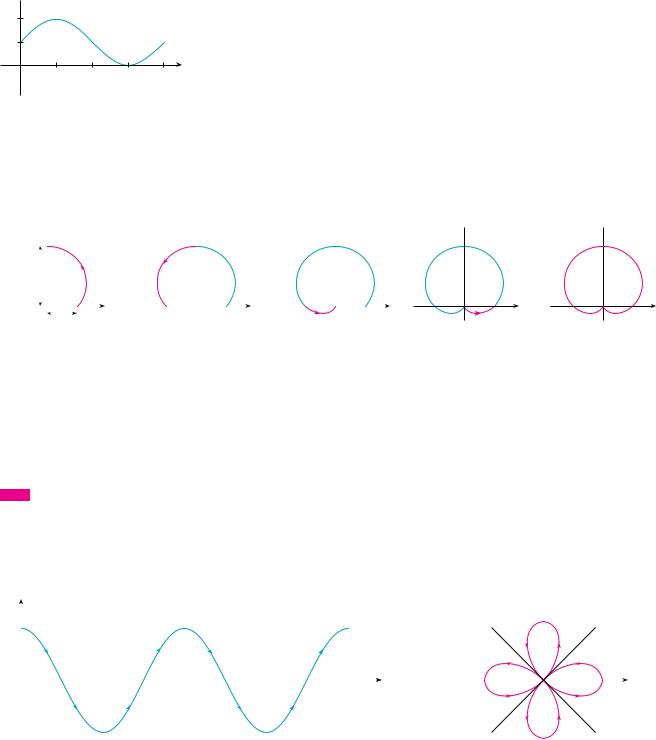
r 1 sin in Cartesian coordinates in Figure 10 by shifting the sine curve up one unit. This enables us to read at a glance the values of r that correspond to increasing values of . For instance, we see that as increases from 0 to 2, r (the distance from O) increases from 1 to 2, so we sketch the corresponding part of the polar curve in Figure 11(a). As increases from 2 to , Figure 10 shows that r decreases from 2 to 1, so we sketch the next part of the curve as in Figure 11(b). As increases from to 3 2,

r decreases from 1 to 0 as shown in part (c). Finally, as increases from 3 2 to 2 , r increases from 0 to 1 as shown in part (d). If we let increase beyond 2 or decrease

beyond 0, we would simply retrace our path. Putting together the parts of the curve from Figure 11(a)–(d), we sketch the complete curve in part (e). It is called a cardioid, because it’s shaped like a heart.

FIGURE 11 Stages in sketching the cardioid r=1+sin ¨

EXAMPLE 8 Sketch the curve r cos 2

OO

M

.

TEC Module 10.3 helps you see how polar curves are traced out by showing animations similar to Figures 10–13.

SOLUTION As in Example 7, we first sketch r cos 2 , 0 2 , in Cartesian coordinates in Figure 12. As increases from 0 to 4, Figure 12 shows that r decreases from 1 to 0 and so we draw the corresponding portion of the polar curve in Figure 13 (indicated by !). As increases from 4 to 2, r goes from 0 to 1. This means that the distance from O increases from 0 to 1, but instead of being in the first quadrant this portion of the polar curve (indicated by @) lies on the opposite side of the pole in the third quadrant. The remainder of the curve is drawn in a similar fashion, with the arrows and numbers indicating the order in which the portions are traced out. The resulting curve has four loops and is called a four-leaved rose.

TANGENTS TO POLAR CURVES

To find a tangent line to a polar curve r parametric equations as

x r cos f cos

f

, we regard as a parameter and write its

y r sin f sin

3

dy dx

dy

d

dx

d

dr

d dr

d

sin r cos

cos r sin

dy

dx

tan

”21 , 7π6 ’ ”21 , 11π6 ’

FIGURE 15

SECTION 10.3 POLAR COORDINATES |||| 645

For instance, in Example 8 we found that r cos 2 0 when 4 or 3 4. This means that the lines 4 and 3 4 (or y x and y x) are tangent lines to r cos 2 at the origin.

M

x r cos y r sin

1 sin cos cos

1 sin sin sin

12 sin 2

sin2

Then we would have

dy dy d dx dx d

sin 2

FIGURE 16 r=sin@(2.4¨)+cos$(2.4¨)