4.3 HOW DERIVATIVES AFFECT THE SHAPE OF A GRAPH

Добавил:

PavelEngineer Опубликованный материал нарушает ваши авторские права? Сообщите нам.

Вуз:

Севастопольский Государственный Университет

Предмет:

[НЕСОРТИРОВАННОЕ]

Файл:

[James_Stewart]_Single_Variable_Calculus_Early_Tr(BookFi).pdf

Скачиваний:

Добавлен:

30.12.2019

Размер:

18.09 Mб

Скачать

☆

<<< < Предыдущая 19 20 21 22 23 24 25 26 27 28 29 3031 / 9131 32 33 34 35 36 37 38 39 40 41 42 43 > Следующая >>>

SECTION 4.3 HOW DERIVATIVES AFFECT THE SHAPE OF A GRAPH |||| 287

x4 ' x3 ' 1

x 2 tan%1 x

x 2 ' x ' 1

Many of the applications of calculus depend on our ability to deduce facts about a function f from information concerning its derivatives. Because f '"x# represents the slope of the curve y ! f "x# at the point "x, f "x##, it tells us the direction in which the curve proceeds

y at each point. So it is reasonable to expect that information about f '"x# will provide us with D information about f "x#.

	B			WHAT DOES f ' SAY ABOUT f ?
				WHAT DOES f ' SAY ABOUT f ?
				To see how the derivative of f can tell us where a function is increasing or decreasing, look
	C			at Figure 1. (Increasing functions and decreasing functions were deﬁned in Section 1.1.)
A	C			Between A and B and between C and D, the tangent lines have positive slope and so
				f '"x# ) 0. Between B and C, the tangent lines have negative slope and so f '"x# * 0. Thus
0		x
0		x		it appears that f increases when f '"x# is positive and decreases when f '"x# is negative. To

FIGURE 1				prove that this is always the case, we use the Mean Value Theorem.
FIGURE 1

					INCREASING/DECREASING TEST
N Let’s abbreviate the name of this test to					(a)	If f '"x# ) 0 on an interval, then	f	is increasing on that interval.
the I/D Test.					(b)	If f '"x# * 0 on an interval, then	f	is decreasing on that interval.
					(b)	If f '"x# * 0 on an interval, then	f	is decreasing on that interval.

				P R O O F
				(a) Let x1 and x2 be any two numbers in the interval with x1 * x2. According to the deﬁ-
				nition of an increasing function (page 20) we have to show that f "x1# * f "x2 #.
					Because we are given that f '"x# ) 0, we know that f is differentiable on %x1, x2 &. So,
				by the Mean Value Theorem there is a number c between x1 and x2 such that
			1			f "x2 # # f "x1# ! f '"c#"x2 # x1#
				Now f '"c# ) 0 by assumption and x2 # x1 ) 0 because x1 * x2. Thus the right side of
				Equation 1 is positive, and so
						f "x2 # # f "x1# ) 0		or	f "x1# * f "x2 #
				This shows that f is increasing.
					Part (b) is proved similarly.				M
					EXAMPLE 1 Find where the function f "x# ! 3x4 # 4x3 # 12x2 % 5 is increasing and
				V
				where it is decreasing.
				SOLUTION		f '"x# ! 12x3 # 12x2 # 24x ! 12x"x # 2#"x % 1#
				To use the I'D Test we have to know where f '"x# ) 0 and where f '"x# * 0. This
				depends on the signs of the three factors of f '"x#, namely, 12x, x # 2, and x % 1. We
				divide the real line into intervals whose endpoints are the critical numbers #1, 0, and
				2 and arrange our work in a chart. A plus sign indicates that the given expression is posi-
				tive, and a minus sign indicates that it is negative. The last column of the chart gives the

288 |||| CHAPTER 4 APPLICATIONS OF DIFFERENTIATION

	20
_2	3
	_30

FIGURE 2

conclusion based on the I'D Test. For instance, f '"x# * 0 for 0 * x * 2, so f is decreasing on (0, 2). (It would also be true to say that f is decreasing on the closed interval %0, 2&.)

	Interval	12x	x # 2	x % 1	f '"x#	f

	x * #1	#	#	#	#	decreasing on (#-, #1)
#1	* x * 0	#	#	%	%	increasing on (#1, 0)
0	* x * 2	%	#	%	#	decreasing on (0, 2)
	x ) 2	%	%	%	%	increasing on (2, -)

The graph of f shown in Figure 2 conﬁrms the information in the chart.							M

Recall from Section 4.1 that if f has a local maximum or minimum at c, then c must be a critical number of f (by Fermat’s Theorem), but not every critical number gives rise to a maximum or a minimum. We therefore need a test that will tell us whether or not f has a local maximum or minimum at a critical number.

You can see from Figure 2 that f "0# ! 5 is a local maximum value of f because f increases on "#1, 0# and decreases on "0, 2#. Or, in terms of derivatives, f '"x# ) 0 for

#1 * x * 0 and f '"x# * 0 for 0 * x * 2. In other words, the sign of f '"x# changes from positive to negative at 0. This observation is the basis of the following test.

THE FIRST DERIVATIVE TEST Suppose that c is a critical number of a continuous function f.

(a)If f ' changes from positive to negative at c, then f has a local maximum at c.

(b)If f ' changes from negative to positive at c, then f has a local minimum at c.

(c)If f ' does not change sign at c (for example, if f ' is positive on both sides of c or negative on both sides), then f has no local maximum or minimum at c.

The First Derivative Test is a consequence of the I'D Test. In part (a), for instance, since

the sign of f '"x# changes from positive to negative at c,

f is increasing to the left of c and

decreasing to the right of c. It follows that

has a local maximum at c.

It is easy to remember the First Derivative Test by visualizing diagrams such as those

in Figure 3.

f»(x)>0

f»(x)<0

f»(x)>0

f»(x)<0

f»(x)>0

(a) Local maximum

(b) Local minimum

(d) No maximum or minimum

FIGURE 3

SECTION 4.3 HOW DERIVATIVES AFFECT THE SHAPE OF A GRAPH |||| 289

N The + signs in the table come from the fact

that t'"x# ) 0 when cos x ) #12. From the graph of y ! cos x, this is true in the indicated

intervals.

FIGURE 4

V EXAMPLE 2 Find the local minimum and maximum values of the function f in Example 1.

SOLUTION From the chart in the solution to Example 1 we see that f '"x# changes from negative to positive at #1, so f "#1# ! 0 is a local minimum value by the First Derivative Test. Similarly, f 'changes from negative to positive at 2, so f "2# ! #27 is also a local minimum value. As previously noted, f "0# ! 5 is a local maximum value because f '"x#

changes from positive to negative at 0.	M
EXAMPLE 3 Find the local maximum and minimum values of the function
t"x# ! x % 2 sin x	0 , x , 2&

SOLUTION To ﬁnd the critical numbers of t, we differentiate: t'"x# ! 1 % 2 cos x

So t'"x# ! 0 when cos x ! #12 . The solutions of this equation are 2&'3 and 4&'3. Because t is differentiable everywhere, the only critical numbers are 2&'3 and 4&'3 and so we analyze t in the following table.

	Interval	t'"x# ! 1 % 2 cos x	t

0 * x * 2&'3		%	increasing on "0, 2&'3#
2&'3	* x * 4&'3	#	decreasing on "2'3, 4&'3#
4&'3	* x * 2&	%	increasing on "4&'3, 2

Because t'"x# changes from positive to negative at 2&'3, the First Derivative Test tells us that there is a local maximum at 2&'3 and the local maximum value is

% 2,

- !

t"2&'3# !

% 2 sin

% s3

$ 3.83

Likewise, t'"x# changes from negative to positive at 4&'3 and so

t"4&'3# !

% 2 sin

% 2,#

- !

# s3 $ 2.46

is a local minimum value. The graph of t in Figure 4 supports our conclusion.

y=x+2"sin"x

2π

290 |||| CHAPTER 4 APPLIC ATIONS OF DIFFERENTIATION

W H AT D O E S f ! S AY A B O U T f ?

Figure 5 shows the graphs of two increasing functions on !a, b". Both graphs join point A to point B but they look different because they bend in different directions. How can we distinguish between these two types of behavior? In Figure 6 tangents to these curves have been drawn at several points. In (a) the curve lies above the tangents and f is called concave upward on !a, b". In (b) the curve lies below the tangents and t is called concave downward on !a, b".

FIGURE 5

(a)

(b)

FIGURE 6

(a) Concave upward

(b) Concave downward

DEFINITION If the graph of f lies above all of its tangents on an interval I, then it is called concave upward on I. If the graph of f lies below all of its tangents on I, it is called concave downward on I.

Figure 7 shows the graph of a function that is concave upward (abbreviated CU) on the intervals !b, c", !d, e", and !e, p" and concave downward (CD) on the intervals !a, b", !c, d", and ! p, q".

y		D
		D
B	C	P
	C

0 a

FIGURE 7

Let’s see how the second derivative helps determine the intervals of concavity. Looking at Figure 6(a), you can see that, going from left to right, the slope of the tangent increases.

SECTION 4.3 HOW DERIVATIVES AFFECT THE SHAPE OF A GRAPH |||| 291

This means that the derivative f " is an increasing function and therefore its derivative f ! is positive. Likewise, in Figure 6(b) the slope of the tangent decreases from left to right, so f " decreases and therefore f ! is negative. This reasoning can be reversed and suggests that the following theorem is true. A proof is given in Appendix F with the help of the Mean Value Theorem.

CONCAVITY TEST

(a)If f !!x" $ 0 for all x in I, then the graph of f is concave upward on I.

(b)If f !!x" # 0 for all x in I, then the graph of f is concave downward on I.

EXAMPLE 4 Figure 8 shows a population graph for Cyprian honeybees raised in an apiary. How does the rate of population increase change over time? When is this rate highest? Over what intervals is P concave upward or concave downward?

	P
	P
	80
	80
Number of bees	60
	60

(in thousands)	40


	20
	20

	0	3	6	9	12	15	18	t
FIGURE 8				Time (in weeks)
FIGURE 8				Time (in weeks)

SOLUTION By looking at the slope of the curve as t increases, we see that the rate of increase of the population is initially very small, then gets larger until it reaches a maximum at about t ! 12 weeks, and decreases as the population begins to level off. As the population approaches its maximum value of about 75,000 (called the carrying capacity), the rate of increase, P"!t", approaches 0. The curve appears to be concave upward on (0, 12) and concave downward on (12, 18). M

In Example 4, the population curve changed from concave upward to concave downward at approximately the point (12, 38,000). This point is called an inﬂection point of the curve. The signiﬁcance of this point is that the rate of population increase has its maximum value there. In general, an inﬂection point is a point where a curve changes its direction of concavity.

DEFINITION A point P on a curve y ! f !x" is called an inﬂection point if f is continuous there and the curve changes from concave upward to concave downward or from concave downward to concave upward at P.

For instance, in Figure 7, B, C, D, and P are the points of inﬂection. Notice that if a curve has a tangent at a point of inﬂection, then the curve crosses its tangent there.

In view of the Concavity Test, there is a point of inﬂection at any point where the second derivative changes sign.

292 \|\|\|\|		CHAPTER 4		APPLIC ATIONS OF DIFFERENTIATION
							EXAMPLE 5 Sketch a possible graph of a function f that satisﬁes the following
						V
						conditions:
							!i" f "!x" $ 0 on !%&, 1", f "!x" # 0 on !1, &"
							!ii" f !!x" $ 0 on !%&, %2" and !2, &", f !!x" # 0 on !%2, 2"
							!iii" lim f !x" ! %2,	lim f !x" ! 0
							x l%&	x l&
		y				SOLUTION Condition (i) tells us that f is increasing on !%&, 1" and decreasing on !1, &".
						Condition (ii) says that f		is concave upward on !%&, %2" and !2, &", and concave down-


						ward on !%2, 2". From condition (iii) we know that the graph of f has two horizontal
						asymptotes: y ! %2 and y ! 0.
-2		0	1	2	x	asymptotes: y ! %2 and y ! 0.
-2		0	1	2	x		We ﬁrst draw the horizontal asymptote y ! %2 as a dashed line (see Figure 9). We
						then draw the graph of f		approaching this asymptote at the far left, increasing to its maxi-
	y=_2					mum point at x ! 1 and decreasing toward the x-axis at the far right. We also make sure
						that the graph has inﬂection points when x ! %2 and 2. Notice that we made the curve
FIGURE 9						bend upward for x # %2 and x $ 2, and bend downward when x is between %2 and 2.

y			f
			f
	P		Ä
	f »(c)=0	f(c)	Ä
		f(c)
0	c	x	x

FIGURE 10

f á(c)>0, f is concave upward

Another application of the second derivative is the following test for maximum and minimum values. It is a consequence of the Concavity Test.

THE SECOND DERIVATIVE TEST Suppose f ! is continuous near c.

(a)If f "!c" ! 0 and f !!c" $ 0, then f has a local minimum at c.

(b)If f "!c" ! 0 and f !!c" # 0, then f has a local maximum at c.

For instance, part (a) is true because f !!x" $ 0 near c and so f is concave upward near c. This means that the graph of f lies above its horizontal tangent at c and so f has a local minimum at c. (See Figure 10.)

V EXAMPLE 6 Discuss the curve y ! x4 % 4x3 with respect to concavity, points of inﬂection, and local maxima and minima. Use this information to sketch the curve.

SOLUTION If f !x" ! x4 % 4x3, then

f "!x" ! 4x3 % 12x2 ! 4x2!x % 3"

f !!x" ! 12x2 % 24x ! 12x!x % 2"

To ﬁnd the critical numbers we set f "!x" ! 0 and obtain x ! 0 and x ! 3. To use the Second Derivative Test we evaluate f ! at these critical numbers:

f !!0" ! 0

f !!3" ! 36

$ 0

Since f "!3" ! 0 and f !!3" $ 0, f !3" ! %27 is a local minimum. Since f !!0" ! 0, the Second Derivative Test gives no information about the critical number 0. But since

f "!x" # 0 for x # 0 and also for 0 # x # 3, the First Derivative Test tells us that f does not have a local maximum or minimum at 0. [In fact, the expression for f "!x" shows that f decreases to the left of 3 and increases to the right of 3.]

y=x$-4þ

(0,!0)

inﬂection

2 3

points

(2,!_16)

(3,!_27)

FIGURE 11

N Try reproducing the graph in Figure 12 with a graphing calculator or computer. Some machines produce the complete graph, some produce only the portion to the right of the y-axis, and some produce only the portion

between x ! 0 and x ! 6. For an explanation and cure, see Example 7 in Section 1.4. An equivalent expression that gives the correct graph is

y ! !x 2 "1#3 ! % 66 %% xx % % 6 % x %1#3

4(4,!2%?#)

y=x@?#(6-x)!?#

FIGURE 12

SECTION 4.3 HOW DERIVATIVES AFFECT THE SHAPE OF A GRAPH |||| 293

Since f !!x" ! 0 when x ! 0 or 2, we divide the real line into intervals with these numbers as endpoints and complete the following chart.

Interval		f !!x" ! 12x!x % 2"	Concavity

(%&, 0)		'	upward
(0,	2)	%	downward
(2,	&)	'	upward

The point !0, 0" is an inﬂection point since the curve changes from concave upward to

concave downward there. Also, !2, %16" is an inﬂection point since the curve changes
from concave downward to concave upward there.
Using the local minimum, the intervals of concavity, and the inﬂection points, we
sketch the curve in Figure 11.	M

N OT E The Second Derivative Test is inconclusive when f !!c" ! 0. In other words, at such a point there might be a maximum, there might be a minimum, or there might be neither (as in Example 6). This test also fails when f !!c" does not exist. In such cases the First Derivative Test must be used. In fact, even when both tests apply, the First Derivative Test is often the easier one to use.

EXAMPLE 7 Sketch the graph of the function f !x" ! x2#3!6 % x"1#3.

SOLUTION You can use the differentiation rules to check that the ﬁrst two derivatives are

	4 % x	%8
f "!x" !		f !!x" !
	x1#3!6 % x"2#3		x4#3!6 % x"5#3

Since f "!x" ! 0 when x ! 4 and f "!x" does not exist when x ! 0 or x ! 6, the critical numbers are 0, 4, and 6.

Interval		4 % x	x1#3	!6 % x"2#3	f "!x"	f
x # 0		'	%	'	%	decreasing on (%&, 0)
0 # x # 4		'	'	'	'	increasing on (0, 4)
4 # x #	6	%	'	'	%	decreasing on (4, 6)
x $	6	%	'	'	%	decreasing on (6, &)

To ﬁnd the local extreme values we use the First Derivative Test. Since f " changes from negative to positive at 0, f !0" ! 0 is a local minimum. Since f " changes from positive to negative at 4, f !4" ! 25#3 is a local maximum. The sign of f " does not change at 6, so there is no minimum or maximum there. (The Second Derivative Test could be used at 4, but not at 0 or 6 since f ! does not exist at either of these numbers.)

Looking at the expression for f !!x" and noting that x4#3 ( 0 for all x, we have

f !!x" # 0 for x # 0 and for 0 # x # 6 and f !!x" $ 0 for x $ 6. So f is concave downward on !%&, 0" and !0, 6" and concave upward on !6, &", and the only inﬂection point

is !6, 0". The graph is sketched in Figure 12. Note that the curve has vertical tangents at
!0, 0" and !6, 0" because % f "!x" % l & as x l 0 and as x l 6.	M

EXAMPLE 8 Use the ﬁrst and second derivatives of f !x" ! e1#x, together with asymptotes, to sketch its graph.

SOLUTION Notice that the domain of f is $x % x " 0&, so we check for vertical asymptotes by computing the left and right limits as x l 0. As x l 0', we know that t ! 1#x l &,

294 |||| CHAPTER 4 APPLIC ATIONS OF DIFFERENTIATION

TEC In Module 4.3 you can practice using graphical information about f " to determine the shape of the graph of f.

lim e1#x ! lim et ! &

x l0' t l&

and this shows that x ! 0 is a vertical asymptote. As x l 0%, we have t ! 1#x l %&, so

lim e1#x ! lim et ! 0

x l0% t l%&

As x l )&, we have 1#x l 0 and so

lim e1#x ! e0 ! 1

x l)&

This shows that y ! 1 is a horizontal asymptote.

Now let’s compute the derivative. The Chain Rule gives

e1#x f "!x" ! % x2

Since e1#x $ 0 and x2

$ 0 for all x " 0, we have f "!x" # 0 for all x " 0. Thus f is

decreasing on !%&, 0" and on !0, &". There is no critical number, so the function has no

maximum or minimum. The second derivative is

f !!x" ! %

x2e1#x!%1#x2 " % e1#x!2x"

e1#x!2x ' 1"

Since e1#x $ 0 and x4

$ 0, we have f !!x" $ 0 when x $ %21 !x " 0" and f !!x" # 0

when x # %21 . So the curve is concave downward on

(%&, %21 ) and concave upward on

(%21 , 0) and on !0, &". The inﬂection point is

(%21 , e%2).

To sketch the graph of f we ﬁrst draw the horizontal asymptote y ! 1 (as a dashed

line), together with the parts of the curve near the asymptotes in a preliminary sketch

[Figure 13(a)]. These parts reﬂect the information concerning limits and the fact that f is

decreasing on both !%&, 0" and !0, &". Notice that we have indicated that f !x" l 0 as

x l 0% even though f !0" does not exist. In Figure 13(b) we ﬁnish the sketch by incorpo-

rating the information concerning concavity and the inﬂection point. In Figure 13(c) we

check our work with a graphing device.

y=ä

inﬂection

point

y=1

(a) Preliminary sketch

(b) Finished sketch

FIGURE 13

SECTION 4.3 HOW DERIVATIVES AFFECT THE SHAPE OF A GRAPH |||| 295

4.3E X E R C I S E S

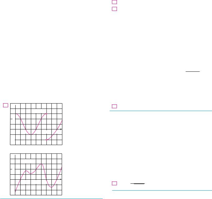
1–2 Use the given graph of f to ﬁnd the following.

(a)The open intervals on which f is increasing.

(b)The open intervals on which f is decreasing.

(c)The open intervals on which f is concave upward.

(d)The open intervals on which f is concave downward.

(e)The coordinates of the points of inﬂection.

1.	y
	1
	0	1	x

2.	y
	1
	0	1	x

3.Suppose you are given a formula for a function f .

(a)How do you determine where f is increasing or decreasing?

(b)How do you determine where the graph of f is concave upward or concave downward?

(c)How do you locate inﬂection points?

4.(a) State the First Derivative Test.

(b)State the Second Derivative Test. Under what circumstances is it inconclusive? What do you do if it fails?

5–6 The graph of the derivative f " of a function f is shown.

(a)On what intervals is f increasing or decreasing?

(b)At what values of x does f have a local maximum or minimum?

5. y			y=f»(x)		6. y				y=f»(x)
5. y					6. y


	0	2	4	6 x		0	2	4		6 x

7.The graph of the second derivative f ! of a function f is shown. State the x-coordinates of the inﬂection points of f . Give reasons for your answers.

y=fá(x)

8 x

8.The graph of the ﬁrst derivative f "of a function f is shown.

(a)On what intervals is f increasing? Explain.

(b)At what values of x does f have a local maximum or minimum? Explain.

(c)On what intervals is f concave upward or concave downward? Explain.

(d)What are the x-coordinates of the inﬂection points of f ?

Why?

y=f»(x)

9–18

(a)Find the intervals on which f is increasing or decreasing.

(b)Find the local maximum and minimum values of f .

(c)Find the intervals of concavity and the inﬂection points.

9.f !x" ! 2x3 ' 3x2 % 36x

10.f !x" ! 4x3 ' 3x2 % 6x ' 1

11.f !x" ! x4 % 2x2 ' 3

12.f !x" ! x2 ' 3

13.	f !x" ! sin x ' cos x,		0 * x * 2+
14.	f !x" ! cos2x % 2 sin x,		0 * x * 2+
15.	f !x" ! e2x ' e%x		16.	f !x" ! x2 ln x
	s				s
17.	f !x" ! !ln x"#	x	18.	f !x" !		x	e%x

19–21 Find the local maximum and minimum values of f using both the First and Second Derivative Tests. Which method do you prefer?

19. f !x" ! x5 % 5x ' 3	20. f !x" !	x
		x2 ' 4

21.f !x" ! x ' s1 % x

22.(a) Find the critical numbers of f !x" ! x4!x % 1"3.

(b)What does the Second Derivative Test tell you about the behavior of f at these critical numbers?

(c)What does the First Derivative Test tell you?

23.Suppose f ! is continuous on !%&, &".

(a)If f "!2" ! 0 and f !!2" ! %5, what can you say about f ?

(b)If f "!6" ! 0 and f !!6" ! 0, what can you say about f ?

24 –29 Sketch the graph of a function that satisﬁes all of the given conditions.

24. f "!x" $ 0 for all x " 1, vertical asymptote x ! 1,

f !!x" $ 0 if x # 1 or x $ 3, f !!x" # 0 if 1 # x # 3

25.f "!0" ! f "!2" ! f "!4" ! 0,

f "!x" $ 0 if x # 0 or 2 # x # 4, f "!x" # 0 if 0 # x # 2 or x $ 4,

f !!x" $ 0 if 1 # x # 3, f !!x" # 0 if x # 1 or x $ 3

296	\|\|\|\| CHAPTER 4	APPLIC ATIONS OF DIFFERENTIATION
26.	f "!1" ! f "!%1" ! 0,			f "!x" # 0 if % x % # 1,
	f "!x" $ 0 if 1 # % x % # 2, f "!x" ! %1 if % x % $ 2,
	f !!x" # 0 if %2 # x # 0,					inﬂection point !0, 1"
27.	f "!x" $ 0 if % x % # 2,			f "!x" # 0 if % x % $ 2,
	x l2	%	f	"!x"	%	! &, f !!x" $ 0 if x " 2
	f "!%2" ! 0, lim
28.	f "!x" $ 0 if % x % # 2,			f "!x" # 0 if % x % $ 2,
	f "!2" ! 0, lim f !x" ! 1,					f !%x" ! %f !x",
	x l&

f !!x" # 0 if 0 # x # 3, f !!x" $ 0 if x $ 3

29.f"!x" # 0 and f !!x" # 0 for all x

30.Suppose f!3" ! 2, f "!3" ! 12, and f "!x" $ 0 and f !!x" # 0 for all x.

(a)Sketch a possible graph for f.

(b)How many solutions does the equation f !x" ! 0 have? Why?

(c)Is it possible that f "!2" ! 13 ? Why?

31–32 The graph of the derivative f " of a continuous function f is shown.

(a)On what intervals is f increasing or decreasing?

(b)At what values of x does f have a local maximum or minimum?

(c)On what intervals is f concave upward or downward?

(d)State the x-coordinate(s) of the point(s) of inﬂection.

(e)Assuming that f !0" ! 0, sketch a graph of f.

31.y

y=f»(x)

8 x

32.y

y=f»(x)

8 x

33– 44

(a)Find the intervals of increase or decrease.

(b)Find the local maximum and minimum values.

(c)Find the intervals of concavity and the inﬂection points.

(d)Use the information from parts (a)–(c) to sketch the graph. Check your work with a graphing device if you have one.

33.	f !x" ! 2x3 % 3x2 % 12x		34.	f !x" ! 2 ' 3x % x3
35.	f !x" ! 2 ' 2x2 % x4		36.	t!x" ! 200 ' 8x3 ' x4
37.	h!x" ! !x ' 1"5 % 5x % 2		38.	h!x" ! x5 % 2x3 ' x
39.	A!x" ! xs		40.	B!x" ! 3x2# 3 % x
		x ' 3
41.	C!x" ! x1# 3!x ' 4"		42.	f !x" ! ln!x4 ' 27"
43.	f !," ! 2 cos , ' cos2,,		0 * , * 2+
44.	f!t" ! t ' cos t, %2+ * t * 2+

45–52

(a)Find the vertical and horizontal asymptotes.

(b)Find the intervals of increase or decrease.

(c)Find the local maximum and minimum values.

(d)Find the intervals of concavity and the inﬂection points.

(e)Use the information from parts (a)–(d) to sketch the graph

of f.

45.	f !x" !		x2
		x2 % 1
47.	f !x" ! s			% x
			x2 ' 1
48.	f !x" ! x tan x, %+#2 # x #
49.	f !x" ! ln!1 % ln x"
51.	f !x" ! e%1#! x'1"

46. f !x" ! !x % 2"2

+#2
50. f !x" !	ex
50. f !x" !	1 ' ex

52. f !x" ! earctan x

53. Suppose the derivative of a function f is

f "!x" ! !x ' 1"2!x % 3"5!x % 6"4. On what interval is f increasing?

54.Use the methods of this section to sketch the curve

y ! x3 % 3a2x ' 2a3, where a is a positive constant. What do the members of this family of curves have in common? How do they differ from each other?

;55–56

(a)Use a graph of f to estimate the maximum and minimum values. Then ﬁnd the exact values.

(b)Estimate the value of x at which f increases most rapidly. Then ﬁnd the exact value.

	x ' 1
55.	f !x" ! sx2 ' 1	56. f ! x" ! x2 e%x

;57–58

(a)Use a graph of f to give a rough estimate of the intervals of concavity and the coordinates of the points of inﬂection.

(b)Use a graph of f ! to give better estimates.

57. f !x" ! cos x ' 12 cos 2x, 0 * x * 2+

SECTION 4.3 HOW DERIVATIVES AFFECT THE SHAPE OF A GRAPH |||| 297

58. f !x" ! x3!x % 2"4

CAS 59–60 Estimate the intervals of concavity to one decimal place by using a computer algebra system to compute and graph f !.

61.A graph of a population of yeast cells in a new laboratory culture as a function of time is shown.

(a)Describe how the rate of population increase varies.

(b)When is this rate highest?

(c)On what intervals is the population function concave upward or downward?

(d)Estimate the coordinates of the inﬂection point.

	700
	700
	600
	600
Number	500
	500
	400
of
of
yeast cells	300
yeast cells	300
	200
	200
	100
	100

	0	2	4	6	8	10	12	14	16	18
					Time (in hours)
					Time (in hours)

62.Let f !t" be the temperature at time t where you live and suppose that at time t ! 3 you feel uncomfortably hot. How do you feel about the given data in each case?

(a) f "!3" ! 2,	f !!3" ! 4		(b) f "!3" ! 2,	f !!3" ! %4
(c) f "!3" ! %2,	f !!3" !	4	(d) f "!3" ! %2,	f !!3" ! %4

63.Let K!t" be a measure of the knowledge you gain by studying for a test for t hours. Which do you think is larger,

K!8" % K!7" or K!3" % K!2"? Is the graph of K concave upward or concave downward? Why?

64.Coffee is being poured into the mug shown in the ﬁgure at a constant rate (measured in volume per unit time). Sketch a rough graph of the depth of the coffee in the mug as a function of time. Account for the shape of the graph in terms of concavity. What is the signiﬁcance of the inﬂection point?

;65. A drug response curve describes the level of medication in the bloodstream after a drug is administered. A surge function S!t" ! At pe%kt is often used to model the response curve, reﬂecting an initial surge in the drug level and then a more gradual decline. If, for a particular drug, A ! 0.01, p ! 4, k ! 0.07, and t is measured in minutes, estimate the times corresponding to the inﬂection points and explain their signiﬁcance. If you have a graphing device, use it to graph the drug response curve.

66.The family of bell-shaped curves

occurs in probability and statistics, where it is called the normal density function. The constant . is called the mean and the positive constant - is called the standard deviation. For simplicity, let’s scale the function so as to remove the factor 1#(-s2+ ) and let’s analyze the special case where . ! 0. So we study the function

2	#!2		2	"
f !x" ! e%x	#!2	-		"
		-

(a) Find the asymptote, maximum value, and inﬂection points of f.

(b) What role does - play in the shape of the curve?

;(c) Illustrate by graphing four members of this family on the same screen.

67.Find a cubic function f !x" ! ax3 ' bx2 ' cx ' d that has a local maximum value of 3 at %2 and a local minimum value of 0 at 1.

68.For what values of the numbers a and b does the function

f !x" ! axebx2 have the maximum value f !2" ! 1?

69.Show that the curve y ! !1 ' x"#!1 ' x2" has three points of inﬂection and they all lie on one straight line.

70.Show that the curves y ! e%x and y ! %e%x touch the curve y ! e%x sin x at its inﬂection points.

71.Suppose f is differentiable on an interval I and f "!x" $ 0 for all numbers x in I except for a single number c. Prove that f is increasing on the entire interval I.

72– 74 Assume that all of the functions are twice differentiable and the second derivatives are never 0.

72.(a) If f and t are concave upward on I, show that f ' t is concave upward on I.

(b)If f is positive and concave upward on I, show that the function t!x" ! ' f !x"( 2 is concave upward on I.

73.(a) If f and t are positive, increasing, concave upward functions on I, show that the product function ft is concave upward on I.

(b)Show that part (a) remains true if f and t are both decreasing.

298 |||| CHAPTER 4 APPLIC ATIONS OF DIFFERENTIATION

74.

75.

76.

77.

;78.

(c)Suppose f is increasing and t is decreasing. Show, by giving three examples, that ft may be concave upward, concave downward, or linear. Why doesn’t the argument in parts (a) and (b) work in this case?

Suppose f and t are both concave upward on !%&, &". Under what condition on f will the composite function h!x" ! f ! t!x"" be concave upward?

Show that tan x $ x for 0 # x # +#2. [Hint: Show that f !x" ! tan x % x is increasing on !0, +#2".]

(a)Show that ex ( 1 ' x for x ( 0.

(b)Deduce that ex ( 1 ' x ' 12 x2 for x ( 0.

(c)Use mathematical induction to prove that for x ( 0 and any positive integer n,

ex ( 1 ' x ' x2 ' 0 0 0 ' xn

2! n!

Show that a cubic function (a third-degree polynomial) always has exactly one point of inﬂection. If its graph has three x-intercepts x1, x2, and x3, show that the x-coordinate of the inﬂection point is !x1 ' x2 ' x3 "#3.

For what values of c does the polynomial

P!x" ! x4 ' cx3 ' x2 have two inﬂection points? One inﬂection point? None? Illustrate by graphing P for several values of c. How does the graph change as c decreases?

79. Prove that if !c, f !c"" is a point of inﬂection of the graph of f and f ! exists in an open interval that contains c, then f !!c" ! 0. [Hint: Apply the First Derivative Test and Fermat’s Theorem to the function t ! f ".]

80. Show that if f !x" ! x4, then f !!0" ! 0, but !0, 0" is not an inﬂection point of the graph of f .

81. Show that the function t!x" ! x % x % has an inﬂection point at !0, 0" but t!!0" does not exist.

82. Suppose that f / is continuous and f "!c" ! f !!c" ! 0, but

f /!c" $ 0. Does f have a local maximum or minimum at c? Does f have a point of inﬂection at c?

83. The three cases in the First Derivative Test cover the situations one commonly encounters but do not exhaust all possibilities. Consider the functions f, t, and h whose values at 0 are all 0 and, for x " 0,

f!x" ! x4 sin	1	t!x" ! x4 )2		' sin	1	*
	x				x
h!x" ! x4		)%2 ' sin	1	*
			x

(a)Show that 0 is a critical number of all three functions but their derivatives change sign inﬁnitely often on both sides of 0.

(b)Show that f has neither a local maximum nor a local minimum at 0, t has a local minimum, and h has a local maximum.

4.4I N D E T E R M I N AT E F O R M S A N D L’ H O S P I TA L’ S RU L E

Suppose we are trying to analyze the behavior of the function

F!x" ! ln x x % 1

Although F is not deﬁned when x ! 1, we need to know how F behaves near 1. In particular, we would like to know the value of the limit

1	lim	ln x
		x % 1
	x l1

In computing this limit we can’t apply Law 5 of limits (the limit of a quotient is the quotient of the limits, see Section 2.3) because the limit of the denominator is 0. In fact, although the limit in (1) exists, its value is not obvious because both numerator and denominator approach 0 and 00 is not deﬁned.

In general, if we have a limit of the form

	lim	f !x"
		t!x"
	x la

where both f !x" l 0 and t!x" l 0 as x l a, then this limit may or may not exist and is called an indeterminate form of type 00. We met some limits of this type in Chapter 2. For

L’HOSPITAL

L’Hospital’s Rule is named after a

French nobleman, the Marquis de l’Hospital (1661–1704), but was discovered by a Swiss mathematician, John Bernoulli (1667–1748). You might sometimes see l’Hospital spelled as l’Hôpital, but he spelled his own name l’Hospital, as was common in the 17th century. See Exercise 77 for the example that the Marquis used to illustrate his rule. See the project on page 307 for further historical details.

SECTION 4.4 INDETERMINATE FORMS AND L’HOSPITAL’S RULE |||| 299

rational functions, we can cancel common factors:

lim	x2 % x	! lim	x!x % 1"	! lim	x	!	1
	x2 % 1		!x ' 1"!x % 1"		x ' 1		2
x l1		x l1		x l1

We used a geometric argument to show that

lim sin x ! 1

x l0 x

But these methods do not work for limits such as (1), so in this section we introduce a systematic method, known as l’Hospital’s Rule, for the evaluation of indeterminate forms.

Another situation in which a limit is not obvious occurs when we look for a horizontal asymptote of F and need to evaluate the limit

	lim	ln x
2		x % 1
	x l&

It isn’t obvious how to evaluate this limit because both numerator and denominator become large as x l &. There is a struggle between numerator and denominator. If the numerator wins, the limit will be &; if the denominator wins, the answer will be 0. Or there may be some compromise, in which case the answer may be some ﬁnite positive number.

In general, if we have a limit of the form

	lim	f !x"
		t!x"
	x la

where both f !x" l & (or %&) and t!x" l & (or %&), then the limit may or may not exist and is called an indeterminate form of type "#". We saw in Section 2.6 that this type of limit can be evaluated for certain functions, including rational functions, by dividing numerator and denominator by the highest power of x that occurs in the denominator. For instance,

					1
				1 %
lim	x2	% 1	! lim	1 %		x2	!	1 % 0	!	1
lim		' 1	! lim		1		!	2 ' 0	!	2
x l& 2x2		' 1	x l&	2	1			2 ' 0		2
					'
					'	x2

This method does not work for limits such as (2), but l’Hospital’s Rule also applies to this type of indeterminate form.

L’HOSPITAL’S RULE	Suppose f and t are differentiable and t"!x" " 0 on an open
interval I that contains a (except possibly at a). Suppose that
	lim f !x" ! 0		and	lim t!x" ! 0
	x la			x la
or that	lim f !x" ! )&		and	lim t!x" ! )&
	x la			x la
(In other words, we have an indeterminate form of type 00 or &.) Then
	lim	f !x"	! lim	f "!x"
		t!x"		t"!x"
	x la		x la

if the limit on the right side exists (or is & or %&).

300 |||| CHAPTER 4 APPLICATIONS OF DIFFERENTIATION


0	a	x

y y=mÁ(x-a)

y=mª(x-a)


0	a	x

FIGURE 1

N Figure 1 suggests visually why l’Hospital’s Rule might be true. The ﬁrst graph shows two differentiable functions f and t, each of which approaches 0 as x l a. If we were to zoom in toward the point !a, 0", the graphs would start to look almost linear. But if the functions actually were linear, as in the second graph, then their ratio would be

m1!x " a" ! m1 m2!x " a" m2

which is the ratio of their derivatives. This suggests that

lim	f !x"	! lim	f #!x"
	t!x"		t#!x"
x la		x la

| Notice that when using l’Hospital’s Rule we differentiate the numerator and denominator separately. We do not use the Quotient Rule.

N The graph of the function of Example 2 is shown in Figure 2. We have noticed previously that exponential functions grow far more rapidly than power functions, so the result of Example 2 is not unexpected. See also Exercise 69.

NOTE 1 L’Hospital’s Rule says that the limit of a quotient of functions is equal to the limit of the quotient of their derivatives, provided that the given conditions are satisﬁed. It is especially important to verify the conditions regarding the limits of f and t before using l’Hospital’s Rule.

NOTE 2 L’Hospital’s Rule is also valid for one-sided limits and for limits at inﬁnity or negative inﬁnity; that is, “x l a” can be replaced by any of the symbols x l a$, x l a", x l !, or x l "!.

NOTE 3 For the special case in which f !a" ! t!a" ! 0, f # and t# are continuous, and t#!a" " 0, it is easy to see why l’Hospital’s Rule is true. In fact, using the alternative form of the deﬁnition of a derivative, we have

lim

f !x" " f !a"

f #!x"

f #!a"

x " a

lim

x la

! lim

x la t#!x"

t#!a"

lim

t!x" " t!a"

x la

t!x" " t!a"

x " a

x la

x " a

! lim

f !x" " f !a"

! lim

f !x"

t!x" " t!a"

t!x"

x la

It is more difﬁcult to prove the general version of l’Hospital’s Rule. See Appendix F.

EXAMPLE 1 Find lim

ln x

SOLUTION

Since

x l1

x " 1

lim ln x ! ln 1 ! 0

and

lim !x " 1" ! 0

x l1

we can apply l’Hospital’s Rule:

!ln x"

ln x

1#x

lim

! lim

! 1

x " 1

x l1

!x " 1"

x l1

EXAMPLE 2 Calculate lim

x l!

SOLUTION

We have limx l! ex ! ! and limx l! x2 ! !, so l’Hospital’s Rule gives

!ex

lim

! lim

x l!

!x2

x l!

y=	«	Since ex l ! and 2x l ! as x l !, the limit on the right side is also indeterminate,
		but a second application of l’Hospital’s Rule gives
	≈
0	10		x		e	x		e	x
		lim	e	! lim			! lim			! !	M
FIGURE 2			2					2
		x l! x		x l! 2x			x l!

N The graph of the function of Example 3 is shown in Figure 3. We have discussed previously the slow growth of logarithms, so it isn’t surprising that this ratio approaches 0 as x l !. See also Exercise 70.

y= ln"x Îãx

10,000

SECTION 4.4 INDETERMINATE FORMS AND L’HOSPITAL’S RULE |||| 301

3
SOLUTION Since ln x l ! and sx l ! as x l !, l’Hospital’s Rule applies:
	lim	ln x	! lim	1#x
		3		1	"2#3

	x l! sx		x l! 3 x

Notice that the limit on the right side is now indeterminate of type 00. But instead of applying l’Hospital’s Rule a second time as we did in Example 2, we simplify the expression and see that a second application is unnecessary:

FIGURE 3

N The graph in Figure 4 gives visual conﬁrmation of the result of Example 4. If we were to zoom in too far, however, we would get an inaccurate graph because tan x is close to x when x is small. See Exercise 38(d) in Section 2.2.

		y=tan"x- x
		þ
_1		1
_1	0	1
	0

FIGURE 4

ln x

1#x

lim

! lim

! 0

"2#3

x l!

x l! 3 x

x l! sx

EXAMPLE 4 Find lim

tan x " x . (See Exercise 38 in Section 2.2.)

x l0

SOLUTION Noting that both tan x " x l 0 and x3 l 0 as x l 0, we use l’Hospital’s Rule:

lim	tan x " x	! lim	sec2x " 1
	x3		3x2
x l0		x l0

Since the limit on the right side is still indeterminate of type 00, we apply l’Hospital’s Rule again:

	lim sec2x " 1 ! lim				2 sec2x tan x
						6x
	x l0	3x2		x l0
Because limx l0 sec2x ! 1, we simplify the calculation by writing
lim	2 sec2x tan x	!	1	lim sec2x lim		tan x !	1	lim	tan x
	6x						3		x
x l0		3		x l0	x l0	x		x l0

We can evaluate this last limit either by using l’Hospital’s Rule a third time or by writing tan x as !sin x"#!cos x" and making use of our knowledge of trigonometric limits. Putting together all the steps, we get

lim

tan x " x

! lim

sec2x " 1

! lim

2 sec2x tan x

3x2

x l0

lim

tan x

lim

sec

x l0

EXAMPLE 5 Find lim

sin x

" cos x

x l%" 1

SOLUTION If we blindly attempted to use l’Hospital’s Rule, we would get

lim

sin x

! lim

cos x ! "!

x l%" 1 " cos x

x l %"

sin x

This is wrong! Although the numerator sin x l 0 as x l %", notice that the denominator !1 " cos x" does not approach 0, so l’Hospital’s Rule can’t be applied here.

302 |||| CHAPTER 4 APPLICATIONS OF DIFFERENTIATION

The required limit is, in fact, easy to ﬁnd because the function is continuous at %

the denominator is nonzero there:
lim	sin x	!	sin %	!	0	! 0
			1 " cos %		1 " !"1"
x l%" 1 " cos x

and

N Figure 5 shows the graph of the function in Example 6. Notice that the function is undeﬁned at x ! 0; the graph approaches the origin but never quite reaches it.

y=x"ln"x

FIGURE 5

Example 5 shows what can go wrong if you use l’Hospital’s Rule without thinking. Other limits can be found using l’Hospital’s Rule but are more easily found by other methods. (See Examples 3 and 5 in Section 2.3, Example 3 in Section 2.6, and the discussion at the beginning of this section.) So when evaluating any limit, you should consider other methods before using l’Hospital’s Rule.

INDETERMINATE PRODUCTS

If limx la f !x" ! 0 and limx la t!x" ! ! (or "!), then it isn’t clear what the value of limx la f !x"t!x", if any, will be. There is a struggle between f and t. If f wins, the answer will be 0; if t wins, the answer will be ! (or "!). Or there may be a compromise where the answer is a ﬁnite nonzero number. This kind of limit is called an indeterminate form of type 0 # !. We can deal with it by writing the product ft as a quotient:

ft !	f	or	ft !	t
	1#t			1#f

This converts the given limit into an indeterminate form of type 00 or !#! so that we can use l’Hospital’s Rule.

V EXAMPLE 6 Evaluate lim x ln x.

x l0$

SOLUTION The given limit is indeterminate because, as x l 0$, the ﬁrst factor !x" approaches 0 while the second factor !ln x" approaches "!. Writing x ! 1#!1#x", we have 1#x l ! as x l 0$, so l’Hospital’s Rule gives

lim x ln x ! lim		ln x	! lim	1#x		! lim !"x" ! 0	M
		1#x		"1#x	2
x l0$	x l0$		x l0$			x l0$

NOTE In solving Example 6 another possible option would have been to write

lim	x ln x ! lim	x
		1#ln x
x l0$	x l0$

This gives an indeterminate form of the type 0#0, but if we apply l’Hospital’s Rule we get a more complicated expression than the one we started with. In general, when we rewrite an indeterminate product, we try to choose the option that leads to the simpler limit.

INDETERMINATE DIFFERENCES

If limx la f !x" ! ! and limx la t!x" ! !, then the limit

lim $ f !x" " t!x"%

x la

is called an indeterminate form of type !"!. Again there is a contest between f and t. Will the answer be ! ( f wins) or will it be "! (twins) or will they compromise on a ﬁnite number? To ﬁnd out, we try to convert the difference into a quotient (for instance, by using

SECTION 4.4 INDETERMINATE FORMS AND L’HOSPITAL’S RULE |||| 303

a common denominator, or rationalization, or factoring out a common factor) so that we have an indeterminate form of type 00 or !#!.

EXAMPLE 7 Compute lim	!sec x " tan x".
x l! #2"	"
%	"

SOLUTION First notice that sec x l ! and tan x l ! as x l !%#2"", so the limit is indeterminate. Here we use a common denominator:

lim !sec x " tan x" !

lim

sin x

&cos x

cos x '

x l!%#2""

x l! %#2""

lim

1 " sin x

! lim

"cos x

! 0

"sin x

x l! #2"

cos x

x l! #2"

Note that the use of l’Hospital’s Rule is justiﬁed because 1 " sin x l 0 and cos x l 0

as x l !%#2"".

INDETERMINATE POWERS

Several indeterminate forms arise from the limit

lim $ f !x"%t! x"

x la

1.	lim f !x" ! 0	and	lim t!x" ! 0	type 00
	x la		x la
2.	lim f !x" ! !	and	lim t!x" ! 0	type !0
	x la		x la
3.	lim f !x" ! 1	and	lim t!x" ! &!	type 1!
	x la		x la

Each of these three cases can be treated either by taking the natural logarithm:

let y ! $ f !x"%t! x", then ln y ! t!x" ln f !x"

or by writing the function as an exponential:

$ f !x"%t! x" ! et! x" ln f ! x"

(Recall that both of these methods were used in differentiating such functions.) In either method we are led to the indeterminate product t!x" ln f !x", which is of type 0 # !.

EXAMPLE 8 Calculate lim		!1 $ sin 4x"cot x.
	x l0$
SOLUTION	First notice that as x l 0$, we have 1 $ sin 4x l 1 and cot x l !, so the
given limit is indeterminate. Let
			y ! !1 $ sin 4x"cot x
Then	ln y ! ln$!1		$ sin 4x"cot x % ! cot x ln!1				$ sin 4x"
so l’Hospital’s Rule gives
						4 cos 4x
			ln!1 $ sin 4x"
	lim ln y ! lim		ln!1 $ sin 4x"	! lim	1		$ sin 4x	! 4
	lim ln y ! lim		tan x	! lim			sec2x	! 4
	x l0$	x l0$	tan x	x l0$			sec2x

So far we have computed the limit of ln y, but what we want is the limit of y. To ﬁnd this

304 |||| CHAPTER 4 APPLICATIONS OF DIFFERENTIATION

we use the fact that y ! eln y:

N The graph of the function y ! x x, x ' 0, is shown in Figure 6. Notice that although 00 is not deﬁned, the values of the function approach 1 as x l 0$. This conﬁrms the result of Example 9.

_1	0	2
	0

FIGURE 6

4.4EXERCISES

lim !1	$ sin 4x"cot x ! lim y ! lim eln y ! e4	M
x l0$	x l0$ x l0$

EXAMPLE 9 Find lim x x.

x l0$

SOLUTION Notice that this limit is indeterminate since 0x ! 0 for any x ' 0 but x0 ! 1 for any x " 0. We could proceed as in Example 8 or by writing the function as an exponential:

x x ! !eln x "x ! ex ln x

In Example 6 we used l’Hospital’s Rule to show that

lim x ln x ! 0

x l0$

Therefore
lim x x ! lim ex ln x ! e0 ! 1		M
x l0$	x l0$

1– 4 Given that
lim f !x" ! 0	lim t!x" ! 0		lim h!x" ! 1
x la	x la		x la
lim p!x" ! !		lim q! x" ! !
x la		x la

which of the following limits are indeterminate forms? For those that are not an indeterminate form, evaluate the limit where possible.

1.(a) lim

xla

(c)lim

xla

(e)lim

xla

2.(a) lim

xla

(c)lim

xla

3.(a) lim

xla

(c)lim

xla

4.(a) lim

xla

(d)lim

xla

f !x"

t!x" h!x"

p!x" p!x"

q!x"

$ f !x"p!x"% $ p!x"q!x"%

$ f !x" " p!x"%

$ p!x" $ q!x"%

$ f !x"% t! x" (b) lim

x la

$ p!x"% f ! x" (e) lim

x la

(b)lim

x la

(d)lim

x la

(b)lim

x la

(b)lim

x la

$ f !x"% p! x"

$ p!x"%q! x"

f !x"

p!x" p!x"

f !x"

$h!x"p!x"%

$p!x" " q!x"%

(c)lim $h!x"% p! x"

x la

(f)lim q!sx" p!x"

x la

5–64 Find the limit. Use l’Hospital’s Rule where appropriate. If there is a more elementary method, consider using it. If l’Hospital’s Rule doesn’t apply, explain why.


5.	lim	x	2			" 1
5.	lim	x2 " x
	x l1	x2 " x
7.	lim	x	9			" 1
7.	lim	x	5 " 1
	x l1	x	5 " 1
9.	lim						cos x
9.	lim			$			1 " sin x
	x l! %#2"						1 " sin x
11.	lim	et			" 1
11.	lim				t3
	t l0				t3

13.lim tan px x l0 tan qx

15.lim ln x

xl! sx


17.	lim			ln x
				x
	x l0$
19.	lim		ex
			x3
	x l!
21.	lim	ex " 1 " x
					x2
	x l0


6.	lim	x2		$ x " 6
				x " 2
	x l2
8.	lim	xa " 1
		xb " 1
	x l1
10.	lim	sin 4x
	xl0	tan 5x
12.	lim	e3t " 1
				t
	t l0
14.	lim		1 " sin (
				csc (
	(l %# 2
16.	lim	x $ x2
		1 " 2x2
	x l!

18.lim ln ln x

xl! x

20.	lim	ln x
		sin %x
	x l1
22.	lim	ex " 1 " x " 21 x2
			x3
	x l0

23.lim tanh x x l0 tan x

25.	lim	5t " 3t
		t
	t l0
27.	lim	sin"1x
		x
	x l0
29.	lim	1 " cos x
		x2
	x l0

31.lim x $ sin x x l0 x $ cos x

33.lim 1 " x $ ln x x l1 1 $ cos %x

35.	lim	xa " ax $ a " 1
		!x " 1"2
	x l1
37.	lim	cos x " 1 $ 21 x2
		x4
	x l0

39.lim x sin!%#x"

xl!

41.lim cot 2x sin 6x

x l0

43.lim x3e"x 2

xl!

45.	lim ln x tan!%x#2"
	x l1$
	lim		x	"	1
47.		&x " 1			ln x	'
	x l1

49.lim (sx2 $ x " x)

xl!

51.lim !x " ln x"

xl!

53.lim x x2

xl0$

55.lim !1 " 2x"1#x

xl0

	&			3		5	'	x
57. lim		1	$		$
				x		x2
x l!

59.lim x1#x

xl!

61. lim !4x $ 1"cot x

x l0$

SECTION 4.4 INDETERMINATE FORMS AND L’HOSPITAL’S RULE |||| 305

24.lim x " sin x x l0 x " tan x

26. lim	sin x " x
x l0	x3

28.lim !ln x"2

xl! x

30.	lim	cos mx " cos nx
	x l0			x2
32.	lim		x
32.	lim	tan"1!4x"
	x l0	tan"1!4x"

34.	lim	s	x2	$ 2
34.	lim
	x l! s2x2			$ 1

36.lim ex " e"x " 2x x l0 x " sin x

38. lim	cos x ln!x " a"
x la$	ln!ex " ea "

40. lim x2ex

x l"!

42. lim sin x ln x

x l0$

44.lim !1 " tan x" sec x

xl%# 4

46.lim x tan!1#x"

xl!

48.lim !csc x " cot x"

xl0

x l0 &		x '
50. lim	cot x "	1

52.lim !xe1#x " x"

xl!

54.lim !tan 2x"x

xl0$

56.lim &1 $ a 'bx

xl! x

58.lim x!ln 2"#!1 $ ln x"

xl!

60.lim !ex $ x"1#x

xl!

62. lim !2 " x"tan! %x#2"

x l1

63. lim !cos x"1# x	2	64.	lim		2x " 3		2x$1
63. lim !cos x"1# x		64.	lim	&2x $ 5		'
x l0$			x l!	&2x $ 5		'

;65–66 Use a graph to estimate the value of the limit. Then use l’Hospital’s Rule to ﬁnd the exact value.

&2 'x 5x " 4x

65.lim 1 $ 66. lim x x

xl! x x l0 3 " 2

; 67–68 Illustrate l’Hospital’s Rule by graphing both f !x"#t!x" and
	f #!x"#t#!x" near x ! 0 to see that these ratios have the same limit
	as x l 0. Also calculate the exact value of the limit.
67.		f !x" ! ex " 1,	t!x" ! x3	$ 4x
68.		f !x" ! 2x sin x,	t!x" ! sec x " 1

		Prove that
	69.	Prove that
			lim		ex	! !
			lim		xn	! !
			x l!		xn

for any positive integer n. This shows that the exponential function approaches inﬁnity faster than any power of x.

70. Prove that

ln x

lim x p ! 0

x l!

for any number p ' 0. This shows that the logarithmic function approaches ! more slowly than any power of x.

71. What happens if you try to use l’Hospital’s Rule to evaluate

lim

x l! sx2 $ 1

Evaluate the limit using another method.

72.If an object with mass m is dropped from rest, one model for its speed v after t seconds, taking air resistance into account, is

v ! mct !1 " e"ct#m "

where t is the acceleration due to gravity and c is a positive constant. (In Chapter 9 we will be able to deduce this equation from the assumption that the air resistance is proportional to the speed of the object; c is the proportionality constant.)

(a)Calculate limt l ! v. What is the meaning of this limit?

(b)For ﬁxed t, use l’Hospital’s Rule to calculate limc l 0$ v. What can you conclude about the velocity of a falling object in a vacuum?

nr 'nt

306 |||| CHAPTER 4 APPLICATIONS OF DIFFERENTIATION

73. If an initial amount A0 of money is invested at an interest rate r compounded n times a year, the value of the investment after t years is

A ! A0&1 $

If we let n l !, we refer to the continuous compounding of interest. Use l’Hospital’s Rule to show that if interest is compounded continuously, then the amount after t years is

A ! A0ert

74. If a metal ball with mass m is projected in water and the force of resistance is proportional to the square of the velocity, then the distance the ball travels in time t is

s!t" ! mc ln cosh*mttc

where c is a positive constant. Find limc l 0$ s!t".

75.If an electrostatic ﬁeld E acts on a liquid or a gaseous polar dielectric, the net dipole moment P per unit volume is

P!E" !	eE $ e"E		1
		"
	eE " e"E		E
Show that limE l 0$ P!E" ! 0.

76.A metal cable has radius r and is covered by insulation, so that the distance from the center of the cable to the exterior of the insulation is R. The velocity v of an electrical impulse in the cable is

&Rr '2 ln&Rr 'v ! "c

where c is a positive constant. Find the following limits and interpret your answers.

(a) lim v	(b) lim v
R lr$	r l0$

77.The ﬁrst appearance in print of l’Hospital’s Rule was in the book Analyse des Inﬁniment Petits published by the Marquis de l’Hospital in 1696. This was the ﬁrst calculus textbook ever published and the example that the Marquis used in that book to illustrate his rule was to ﬁnd the limit of the function

y ! s2a3x " x4 " as3 aax a " s4 ax3

as x approaches a, where a ' 0. (At that time it was common to write aa instead of a2.) Solve this problem.

78. The ﬁgure shows a sector of a circle with central angle (. Let A!(" be the area of the segment between the chord PR and

the arc PR. Let B!

(

" be the area of the triangle PQR. Find

lim

(l 0$ *!("#+!(".

A(¬)

B(¬)

79.

If f # is continuous, f !2" ! 0, and f #!2" ! 7, evaluate

lim

f !2 $ 3x" $ f !2

$ 5x"

x l0

80. For what values of a and b is the following equation true?

lim

sin 2x

$ a $

! 0

x2 '

x l0 &

If f # is continuous, use l’Hospital’s Rule to show that

81.

lim

f !x $ h" " f !x " h"

! f #!x"

h l0

Explain the meaning of this equation with the aid of a

diagram.

82.

If f ) is continuous, show that

lim

f !x $ h" " 2f !x" $ f !x " h"

! f )!x"

h l0

83.

Let

e"1#x 2

if x " 0

f !x" ! (0

if x ! 0

(a)

Use the deﬁnition of derivative to compute f #!0".

(b)

Show that f has derivatives of all orders that are deﬁned

on !. [Hint: First show by induction that there is a

polynomial pn!x" and a nonnegative integer kn such that

f !n"!x" ! pn!x"f !x"#xkn

for x " 0.]

;84.

Let

)

x if

x " 0

f !x"

! (1)

if x ! 0

(a) Show that f is continuous at 0.

(b) Investigate graphically whether f

is differentiable at 0 by

zooming in several times toward the point !0, 1" on the

graph of f.

reconcile this fact with the appearance of the graphs in

part (b)?

<<< < Предыдущая 19 20 21 22 23 24 25 26 27 28 29 3031 / 9131 32 33 34 35 36 37 38 39 40 41 42 43 > Следующая >>>

Соседние файлы в предмете [НЕСОРТИРОВАННОЕ]

#
05.02.202055.36 Mб19Calculus, 7th Edition ( PDFDrive.com ).pdf
#
30.12.201945.82 Mб41Complete Solutions Manual for_ SINGLE VARIABLE CALCULUS Early Transcendentals 7th Edition by Stewart ( PDFDrive.com ).pdf
#
30.12.201918.09 Mб36[James_Stewart]_Single_Variable_Calculus_Early_Tr(BookFi).pdf