Добавил:

PavelEngineer Опубликованный материал нарушает ваши авторские права? Сообщите нам.

Вуз:

Севастопольский Государственный Университет

Предмет:

[НЕСОРТИРОВАННОЕ]

Файл:

[James_Stewart]_Single_Variable_Calculus_Early_Tr(BookFi).pdf

Скачиваний:

Добавлен:

30.12.2019

Размер:

18.09 Mб

Скачать

☆

<<< < Предыдущая 41 42 43 44 45 46 47 48 49 50 51 5253 / 9153 54 55 56 57 58 59 60 61 62 63 64 65 > Следующая >>>

508 |||| CHAPTER 7 TECHNIQUES OF INTEGRATION

7.8 IMPROPER INTEGRALS

In deﬁning a deﬁnite integral xab f x dx we dealt with a function f deﬁned on a ﬁnite interval a, b and we assumed that f does not have an inﬁnite discontinuity (see Section 5.2). In this section we extend the concept of a deﬁnite integral to the case where the interval is inﬁnite and also to the case where f has an inﬁnite discontinuity in a, b . In either case the integral is called an improper integral. One of the most important applications of this idea, probability distributions, will be studied in Section 8.5.

TYPE 1: INFINITE INTERVALS

Consider the inﬁnite region S that lies under the curve y 1 x2, above the x-axis, and to the right of the line x 1. You might think that, since S is inﬁnite in extent, its area must be inﬁnite, but let’s take a closer look. The area of the part of S that lies to the left of the line x t (shaded in Figure 1) is

t 1		1		t	1
A t y1		dx		1 1
	x2		x		t

Notice that A t 1 no matter how large t is chosen.

≈

x=1

area=1-

FIGURE 1

We also observe that

lim A t lim

t l

The area of the shaded region approaches 1 as t l (see Figure 2), so we say that the area

of the inﬁnite region S is equal to 1 and we write

dx lim

y1 x2

t l y1 x2

area=

area=32

area=54

area=1

5 x

1 2 x

3 x

FIGURE 2

Using this example as a guide, we deﬁne the integral of f (not necessarily a positive function) over an inﬁnite interval as the limit of integrals over ﬁnite intervals.

SECTION 7.8 IMPROPER INTEGRALS |||| 509

1 DEFINITION OF AN IMPROPER INTEGRAL OF TYPE 1

(a) If xat f x dx exists for every number t a, then


f x dx lim		t f x dx
ya	t l ya

provided this limit exists (as a ﬁnite number).

(b) If xtb f x dx exists for every number t b, then

b	f x dx lim	b f x dx
y	t l yt

provided this limit exists (as a ﬁnite number).

The improper integrals xa f x dx and xb f x dx are called convergent if the corresponding limit exists and divergent if the limit does not exist.

y f x dx y f x dx y f x dx

In part (c) any real number a can be used (see Exercise 74).

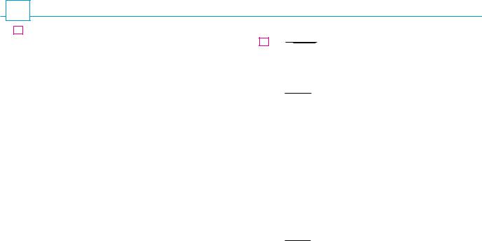
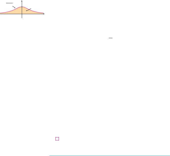
Any of the improper integrals in Deﬁnition 1 can be interpreted as an area provided that

is a positive function. For instance, in case (a) if f x 0 and the integral xa f x dx

is convergent, then we deﬁne the area of the region S x, y x a, 0 y f x in

Figure 3 to be

A S ya

f x dx

This is appropriate because xa f x dx is the limit as t l of the area under the graph of

from a to t.

y=ƒ

FIGURE 3

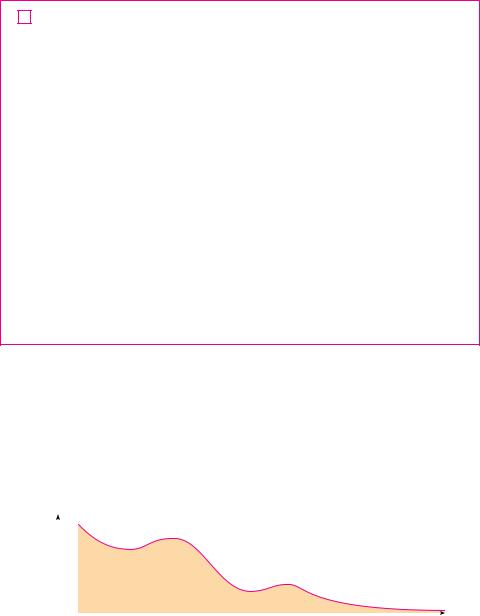
EXAMPLE 1 Determine whether the integral x1 1 x dx is convergent or divergent.

SOLUTION According to part (a) of Deﬁnition 1, we have

dx lim

dx lim ln

x ]t

y1 x

t l y1 x

t l

lim ln t ln 1 lim ln t

t l

The limit does not exist as a ﬁnite number and so the improper integral x1 1 x dx is

divergent.

510 |||| CHAPTER 7 TECHNIQUES OF INTEGRATION

Let’s compare the result of Example 1 with the example given at the beginning of this

section:

≈

dx converges

dx diverges

ﬁnite area

Geometrically, this says that although the curves y 1 x2 and y 1 x look very similar

for x 0, the region under y 1 x2 to the right of x 1 (the shaded region in Figure 4)

has ﬁnite area whereas the corresponding region under y 1 x (in Figure 5) has inﬁnite

area. Note that both 1 x2 and 1 x approach 0 as x l but 1 x2 approaches 0 faster than

FIGURE 4

1 x. The values of 1 x don’t decrease fast enough for its integral to have a ﬁnite value.

EXAMPLE 2 Evaluate y0

xex dx.

SOLUTION Using part (b) of Deﬁnition 1, we have

lim

xex dx

t l yt

We integrate by parts with u x, dv ex dx so that du dx, v ex:

yt0 xex dx xex]0t yt0 ex dx

FIGURE 5

tet 1 et

We know that et l 0 as t l , and by l’Hospital’s Rule we have

TEC In Module 7.8 you can investigate visually and numerically whether several improper integrals are convergent or divergent.


lim tet lim		t	lim	1
lim tet lim			lim
t l	t l e t		t l e t

lim et 0

t l

Therefore

	0	xex dx lim tet 1 et
	y	xex dx lim tet 1 et
	y	t l
		0 1 0 1

EXAMPLE 3 Evaluate y 1 x2 dx.

SOLUTION It’s convenient to choose a 0 in Deﬁnition 1(c):

			1		0	1		1
	y			dx y					dx y0		dx
		1 x2					1 x2			1 x2
We must now evaluate the integrals on the right side separately:
1			dx lim		t		dx	lim tan 1x]0t

y0 1 x2
				t l y0 1 x2					t l
			lim tan 1t tan 1 0 lim tan 1t
				t l					t l

y=1+≈1 y

area=π

FIGURE 6

SECTION 7.8 IMPROPER INTEGRALS |||| 511

0 1

dx lim

lim tan 1x]0t

y 1 x2

t l yt 1 x2

t l

lim

tan 1 0 tan 1t

t l

Since both of these integrals are convergent, the given integral is convergent and

1 x2

Since 1 1 x2	0, the given improper integral can be interpreted as the area of
the inﬁnite region that lies under the curve y 1 1 x2 and above the x-axis (see
Figure 6).	M

EXAMPLE 4 For what values of p is the integral

y x p dx

convergent?

SOLUTION We know from Example 1 that if p 1, then the integral is divergent, so let’s assume that p 1. Then

dx lim

x p dx

x p

t l y1

x p 1

x t

lim

1 x 1

t l p

lim

p t p 1

t l 1

If p

1, then p 1

0, so as t l , t p 1 l and 1 t p 1 l 0. Therefore

if p 1

x p

p 1

and so the integral converges. But if p 1, then p 1 0 and so

t1 p l as t l

t p 1

and the integral diverges.

We summarize the result of Example 4 for future reference:

dx is convergent if p

1 and divergent if p 1.

x p

TYPE 2: DISCONTINUOUS INTEGRANDS

Suppose that f is a positive continuous function deﬁned on a ﬁnite interval a, b but has a vertical asymptote at b. Let S be the unbounded region under the graph of f and above the x-axis between a and b. (For Type 1 integrals, the regions extended indeﬁnitely in a

512 |||| CHAPTER 7 TECHNIQUES OF INTEGRATION

y				horizontal direction. Here the region is inﬁnite in a vertical direction.) The area of the part
y
				of S between a and t (the shaded region in Figure 7) is
		y=ƒ	x=b			t
		y=ƒ	x=b			t
						A t ya f x dx
						A t ya f x dx
				If it happens that A t approaches a deﬁnite number A as t l b , then we say that the
0	a	t b	x	area of the region S is A and we write
FIGURE 7				y	b	t
FIGURE 7						f x dx lim f x dx
						t lb ya
				a		t lb ya

We use this equation to deﬁne an improper integral of Type 2 even when f is not a positive function, no matter what type of discontinuity f has at b.

N Parts (b) and (c) of Deﬁnition 3 are illustrated in Figures 8 and 9 for the case where f x 0 and f has vertical asymptotes at a and c, respectively.

a t

b x

FIGURE 8

0 a

b x

FIGURE 9

y= 1 œ„„„x-„2

area=2œ„3


0	1		2			3			4			5			x

FIGURE 10

3 DEFINITION OF AN IMPROPER INTEGRAL OF TYPE 2

(a) If f is continuous on a, b and is discontinuous at b, then

y	b	t
		f x dx lim f x dx
		t lb ya
a

if this limit exists (as a ﬁnite number).

(b) If f is continuous on a, b and is discontinuous at a, then

b	b
ya	f x dx lim f x dx
ya	t la yt

if this limit exists (as a ﬁnite number).

The improper integral xab f x dx is called convergent if the corresponding limit exists and divergent if the limit does not exist.

(c)	If f has a discontinuity at c, where a c b, and both xac f x dx and
	xcb f x dx are convergent, then we deﬁne
			b		c	b
			ya	f x dx ya		f x dx yc f x dx

	5	1
EXAMPLE 5 Find y2					dx.
		s
		s	x 2
	We note ﬁrst that the given integral is improper because f x 1
SOLUTION							x 2
						s

has the vertical asymptote x 2. Since the inﬁnite discontinuity occurs at the left endpoint of 2, 5 , we use part (b) of Deﬁnition 3:

5 dx

lim

y2 sx 2

t l2 yt

sx 2

lim 2

]t5

x 2

t l2

lim 2(

)

t 2

t l2

Thus the given improper integral is convergent and, since the integrand is positive, we

can interpret the value of the integral as the area of the shaded region in Figure 10.

		SECTION 7.8 IMPROPER INTEGRALS \|\|\|\| 513

	EXAMPLE 6 Determine whether y0	2 sec x dx converges or diverges.
V

SOLUTION Note that the given integral is improper because limx l 2 sec x . Using part (a) of Deﬁnition 3 and Formula 14 from the Table of Integrals, we have

	lim	t sec x dx	lim	ln	sec x tan x	]0t
2 sec x dx	lim	t sec x dx	lim	ln	sec x tan x	]0t
y0	t l 2 y0		t l 2
	lim ln sec t tan t ln 1
	t l 2

because sec t l and tan t l as t l 2 . Thus the given improper integral is

divergent.		M
3	dx
EXAMPLE 7 Evaluate y0		if possible.
	x 1

SOLUTION Observe that the line x 1 is a vertical asymptote of the integrand. Since it occurs in the middle of the interval 0, 3 , we must use part (c) of Deﬁnition 3 with c 1:

x 1

where

1 dx

lim

lim ln

x 1

]0t

y0 x 1

t l1 y0 x 1

t l1

(ln

)

lim

lim ln 1 t

t l1

because 1 t l 0 as t l 1 . Thus x01 dx x 1 is divergent. This implies that

x03 dx x 1 is divergent. [We do not need to evaluate x13 dx x 1 .]

| WARNING If we had not noticed the asymptote x 1 in Example 7 and had instead confused the integral with an ordinary integral, then we might have made the following erroneous calculation:

3 dx		3
y0		ln x 1 ]0	ln 2 ln 1 ln 2
	x 1

This is wrong because the integral is improper and must be calculated in terms of limits. From now on, whenever you meet the symbol xab f x dx you must decide, by looking at the function f on a, b , whether it is an ordinary deﬁnite integral or an improper

integral.

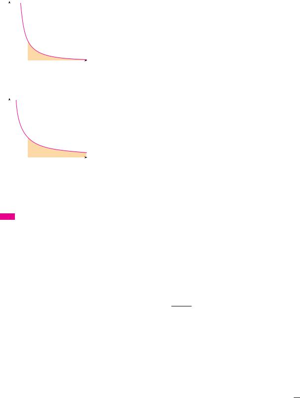
EXAMPLE 8 Evaluate y1 ln x dx.

SOLUTION We know that the function f x ln x has a vertical asymptote at 0 since limx l0 ln x . Thus the given integral is improper and we have

1	1
y0	ln x dx lim ln x dx
y0	t l0 yt

514 |||| CHAPTER 7 TECHNIQUES OF INTEGRATION

0	1	x
	1

area=1

y=ln x

FIGURE 11

y
		f
	g
0	a	x
FIGURE 12

y=e_x2

y=e_x

0	1	x
	1

Now we integrate by parts with u ln x, dv dx, du dx x, and v x:

y1 ln x dx x ln x]1t y1 dx

t t

1 ln 1 t ln t 1 t

t ln t 1 t

To ﬁnd the limit of the ﬁrst term we use l’Hospital’s Rule:


		lim t ln t lim		ln t	lim	1 t	lim t 0
		lim t ln t lim			lim		lim t 0
		t l0	t l0 1 t		t l0 1 t2		t l0
Therefore	1	ln x dx lim t ln t 1 t 0 1 0 1
Therefore	y0	ln x dx lim t ln t 1 t 0 1 0 1
	y0		t l0

Figure 11 shows the geometric interpretation of this result. The area of the shaded region above y ln x and below the x-axis is 1. M

A COMPARISON TEST FOR IMPROPER INTEGRALS

Sometimes it is impossible to ﬁnd the exact value of an improper integral and yet it is important to know whether it is convergent or divergent. In such cases the following theorem is useful. Although we state it for Type 1 integrals, a similar theorem is true for Type 2 integrals.

COMPARISON THEOREM Suppose that f and t are continuous functions with f x t x 0 for x a.

(a)If xa f x dx is convergent, then xa t x dx is convergent.

(b)If xa t x dx is divergent, then xa f x dx is divergent.

We omit the proof of the Comparison Theorem, but Figure 12 makes it seem plausible. If the area under the top curve y f x is ﬁnite, then so is the area under the bottom curve y t x . And if the area under y t x is inﬁnite, then so is the area under y f x . [Note that the reverse is not necessarily true: If xa t x dx is convergent, xa f x dx may or may not be convergent, and if xa f x dx is divergent, xa t x dx may or may not be divergent.]

V EXAMPLE 9 Show that y e x2dx is convergent.

SOLUTION We can’t evaluate the integral directly because the antiderivative of e x2 is not an elementary function (as explained in Section 7.5). We write

	2	1		2			2
y0	e x	dx y0	e x		dx y1	e x	dx

and observe that the ﬁrst integral on the right-hand side is just an ordinary deﬁnite integral. In the second integral we use the fact that for x 1 we have x2 x, so x2 x and therefore e x2 e x. (See Figure 13.) The integral of e x is easy to evaluate:

		t	e x dx lim e 1 e t e 1
FIGURE 13	y1	e x dx lim
		t l y1	t l

SECTION 7.8 IMPROPER INTEGRALS |||| 515

			TABLE 1
	t		x0t e x2 dx
	1	0.7468241328
	2	0.8820813908
	3	0.8862073483
	4	0.8862269118
	5	0.8862269255
	6	0.8862269255

			TABLE 2

	t		x1t 1 e x x dx
2			0.8636306042
5			1.8276735512
10			2.5219648704
100			4.8245541204
1000			7.1271392134
10000			9.4297243064

Thus, taking f x e x and t x e x2 in the Comparison Theorem, we see that
x1 e x2 dx is convergent. It follows that x0 e x2 dx is convergent.	M

In Example 9 we showed that x0 e x2 dx is convergent without computing its value. In Exercise 70 we indicate how to show that its value is approximately 0.8862. In probability theory it is important to know the exact value of this improper integral, as we will see in Section 8.5; using the methods of multivariable calculus it can be shown that the exact

value is

2. Table 1 illustrates the deﬁnition of an improper integral by showing how

the (computer-generated) values of x0t e x2 dx approach2

2 as t becomes large. In fact,

these values converge quite quickly because e x

l 0 very rapidly as x l .

1 e x

EXAMPLE 10 The integral y1

dx is divergent by the Comparison Theorem

because

1 e x

and x1 1 x dx is divergent by Example 1 [or by (2) with p 1].

Table 2 illustrates the divergence of the integral in Example 10. It appears that the values are not approaching any ﬁxed number.

7.8E X E R C I S E S

1. Explain why each of the following integrals is improper.

		4
					2
(a) y1	x4e x	dx		(b)	y0		sec x dx
2		x			0		1
(c) y0			dx	(d)	y			dx
	x2 5x 6					x2 5

2. Which of the following integrals are improper? Why?

2	1				1	1
(a) y1			dx	(b)	y0		dx
	2x 1					2x 1
		sin x			2
(c) y			dx	(d)	y1	ln x 1 dx
		1 x2

3.Find the area under the curve y 1 x3 from x 1 to x t and evaluate it for t 10, 100, and 1000. Then ﬁnd the total area under this curve for x 1.

;4. (a) Graph the functions f x 1 x1.1 and t x 1 x0.9 in the

viewing rectangles 0, 10 by 0, 1 and 0, 100 by 0, 1 .

(b)Find the areas under the graphs of f and t from x 1 to x t and evaluate for t 10, 100, 104, 106, 1010, and 1020.

(c)Find the total area under each curve for x 1, if it exists.

5– 40 Determine whether each integral is convergent or divergent. Evaluate those that are convergent.

	1		0	1
5. y1		dx	6. y		dx
5. y1	3x 1 2	dx	6. y	2x 5	dx

7.y 1 s2 1 w dw

9.y e y 2 dy

11.y 1 x2 dx

	y xe x2 dx
13.


15.	y2 sin d
		x 1
17.	y1			dx
17.	y1	x2 2x		dx

19.	y0	se 5s ds
		ln x
21.	y1		dx
21.		x
		x

23.y 9 x6 dx

	1
25. ye				dx
	x ln x 3
1	3
27. y0			dx
		x5

x2 2 2

10.

y 1

e 2t dt

12.

2 v4 dv

e s

14.

16.

cos

t dt

18.

z 2 3z 2

20.

rer 3 dr

22.

x3e x4 dx

24.

e2x 3

x arctan x

26.

1 x2 2

28.

3 x

516

||||

CHAPTER 7

TECHNIQUES OF INTEGRATION

29.

y 2

30.

x 6 3

x 2

31.

y 2

32.

1 x2

33.

x 1 1 5 dx

34.

4y 1

35.

36.

y 2 csc x dx

x2 6x 5

0 e1 x

e1 x

37. y 1

38.

ln x

39.

y0 z 2 ln z dz

40.

41– 46 Sketch the region and ﬁnd its area (if the area is ﬁnite).

41.S x, y x 1, 0 y ex

42.S x, y x 2, 0 y e x 2

;43. S x, y 0 y 2 x2 9

;44. S x, y x 0, 0 y x x2 9

;45. S x, y 0 x 2, 0 y sec2x

;46. S { x, y 2 x 0, 0 y 1 sx 2 }

;47. (a) If t x sin2x x2, use your calculator or computer to

make a table of approximate values of x1t t x dx for

t 2, 5, 10, 100, 1000, and 10,000. Does it appear that x1 t x dx is convergent?

(b)Use the Comparison Theorem with f x 1 x2 to show that x1 t x dx is convergent.

(c)Illustrate part (b) by graphing f and t on the same screen

for 1 x 10. Use your graph to explain intuitively why x1 t x dx is convergent.

;48. (a) If t x 1 (sx 1), use your calculator or computer to make a table of approximate values of x2t t x dx for t 5, 10, 100, 1000, and 10,000. Does it appear that x2 t x dx is convergent or divergent?

(b)Use the Comparison Theorem with f x 1 sx to show that x2 t x dx is divergent.

(c)Illustrate part (b) by graphing f and t on the same screen

for 2 x 20. Use your graph to explain intuitively why x2 t x dx is divergent.

49–54 Use the Comparison Theorem to determine whether the integral is convergent or divergent.

		x		2 e x
49.	y0		dx	50. y1		dx
		x3 1			x

x 1

arctan x

51.

52.

2 ex

sec

sin

53.

54.

55.

The integral

1 x

is improper for two reasons: The interval 0, is inﬁnite and the integrand has an inﬁnite discontinuity at 0. Evaluate it by expressing it as a sum of improper integrals of Type 2 and Type 1 as follows:

y 1 dx y1 1 dx y 1 dx 0 sx 1 x 0 sx 1 x 1 sx 1 x

56. Evaluate

	1
y2		dx

	xsx2 4

by the same method as in Exercise 55.

57–59 Find the values of p for which the integral converges and evaluate the integral for those values of p.

	1	1			1
57.	y0		dx	58. ye		dx
		xp			x ln x p

59. y1 x p ln x dx

60. (a) Evaluate the integral x0 xne x dx for n 0, 1, 2, and 3.

(b)Guess the value of x0 xne x dx when n is an arbitrary positive integer.

(c)Prove your guess using mathematical induction.

61.(a) Show that x x dx is divergent.

(b)Show that

t	x dx 0
lim	x dx 0
t l y t
This shows that we can’t deﬁne
	t	f x dx
f x dx lim		f x dx
y	t l y t

62. The average speed of molecules in an ideal gas is

	4	M	3 2	2
v			y0	v3e Mv 2RT dv
		2RT

	s

where M is the molecular weight of the gas, R is the gas constant, T is the gas temperature, and v is the molecular speed.

Show that
		M
		8RT
	v

63. We know from Example 1 that the region

x, y x 1, 0 y 1 x has inﬁnite area. Show that by rotating about the x-axis we obtain a solid with ﬁnite volume.

64.Use the information and data in Exercises 29 and 30 of Section 6.4 to ﬁnd the work required to propel a 1000-kg satellite out of the earth’s gravitational ﬁeld.

65.Find the escape velocity v0 that is needed to propel a rocket of mass m out of the gravitational ﬁeld of a planet with mass M and radius R. Use Newton’s Law of Gravitation (see Exer-

cise 29 in Section 6.4) and the fact that the initial kinetic energy of 12 mv02 supplies the needed work.

66.Astronomers use a technique called stellar stereography to determine the density of stars in a star cluster from the observed (two-dimensional) density that can be analyzed from a photograph. Suppose that in a spherical cluster of radius R the density of stars depends only on the distance r from the center of the cluster. If the perceived star density is

given by y s , where s is the observed planar distance from the center of the cluster, and x r is the actual density, it can be shown that

R		2r
y s ys			x r dr
	s
		r2 s2

If the actual density of stars in a cluster is x r 12 R r 2, ﬁnd the perceived density y s .

67.A manufacturer of lightbulbs wants to produce bulbs that last

about 700 hours but, of course, some bulbs burn out faster than others. Let F t be the fraction of the company’s bulbs that burn out before t hours, so F t always lies between 0 and 1.

(a)Make a rough sketch of what you think the graph of F might look like.

(b)What is the meaning of the derivative r t F t ?

(c)What is the value of x0 r t dt? Why?

68.As we saw in Section 3.8, a radioactive substance decays exponentially: The mass at time t is m t m 0 ekt, where m 0 is the initial mass and k is a negative constant. The mean life M of an atom in the substance is

M k y tekt dt

For the radioactive carbon isotope, 14C, used in radiocarbon dating, the value of k is 0.000121. Find the mean life of a 14C atom.

69. Determine how large the number a has to be so that

		1
ya			dx 0.001
	x2	1	dx 0.001
	x2	1

SECTION 7.8 IMPROPER INTEGRALS |||| 517

70.Estimate the numerical value of x0 e x2 dx by writing it as

the sum of x04 e x2 dx and x4 e x2 dx. Approximate the ﬁrst integral by using Simpson’s Rule with n 8 and show that the

second integral is smaller than x4 e 4x dx, which is less than 0.0000001.

71.If f t is continuous for t 0, the Laplace transform of f is the function F deﬁned by

F s y f t e st dt

and the domain of F is the set consisting of all numbers s for which the integral converges. Find the Laplace transforms of the following functions.

(a) f t 1 (b) f t et (c) f t t

72. Show that if 0 f t Meat for t 0, where M and a are constants, then the Laplace transform F s exists for s a.

73.Suppose that 0 f t Meat and 0 f t Keat for t 0, where f is continuous. If the Laplace transform of f t is F s and the Laplace transform of f t is G s , show that

G s sF s f 0 s a

74.If x f x dx is convergent and a and b are real numbers, show that

a		b
y f x dx ya		f x dx y f x dx yb f x dx

75.Show that x0 x2e x 2 dx 12 x0 e x 2 dx.

76.Show that x0 e x 2 dx x01 s ln y dy by interpreting the integrals as areas.

77.Find the value of the constant C for which the integral

		1	C
y	s			dx
0			x 2
		x2 4

converges. Evaluate the integral for this value of C.

78. Find the value of the constant C for which the integral

	x	C
y			dx
0 x2	1	3x 1

converges. Evaluate the integral for this value of C.

79.Suppose f is continuous on 0, and limx l f x 1. Is it possible that x0 f x dx is convergent?

80. Show that if a 1 and b	a 1, then the following inte-
gral is convergent.
	xa

y0 1 xb dx

<<< < Предыдущая 41 42 43 44 45 46 47 48 49 50 51 5253 / 9153 54 55 56 57 58 59 60 61 62 63 64 65 > Следующая >>>

Соседние файлы в предмете [НЕСОРТИРОВАННОЕ]

#
05.02.202055.36 Mб19Calculus, 7th Edition ( PDFDrive.com ).pdf
#
30.12.201945.82 Mб41Complete Solutions Manual for_ SINGLE VARIABLE CALCULUS Early Transcendentals 7th Edition by Stewart ( PDFDrive.com ).pdf
#
30.12.201918.09 Mб36[James_Stewart]_Single_Variable_Calculus_Early_Tr(BookFi).pdf