

- •CONTENTS
- •Preface
- •To the Student
- •Diagnostic Tests
- •1.1 Four Ways to Represent a Function
- •1.2 Mathematical Models: A Catalog of Essential Functions
- •1.3 New Functions from Old Functions
- •1.4 Graphing Calculators and Computers
- •1.6 Inverse Functions and Logarithms
- •Review
- •2.1 The Tangent and Velocity Problems
- •2.2 The Limit of a Function
- •2.3 Calculating Limits Using the Limit Laws
- •2.4 The Precise Definition of a Limit
- •2.5 Continuity
- •2.6 Limits at Infinity; Horizontal Asymptotes
- •2.7 Derivatives and Rates of Change
- •Review
- •3.2 The Product and Quotient Rules
- •3.3 Derivatives of Trigonometric Functions
- •3.4 The Chain Rule
- •3.5 Implicit Differentiation
- •3.6 Derivatives of Logarithmic Functions
- •3.7 Rates of Change in the Natural and Social Sciences
- •3.8 Exponential Growth and Decay
- •3.9 Related Rates
- •3.10 Linear Approximations and Differentials
- •3.11 Hyperbolic Functions
- •Review
- •4.1 Maximum and Minimum Values
- •4.2 The Mean Value Theorem
- •4.3 How Derivatives Affect the Shape of a Graph
- •4.5 Summary of Curve Sketching
- •4.7 Optimization Problems
- •Review
- •5 INTEGRALS
- •5.1 Areas and Distances
- •5.2 The Definite Integral
- •5.3 The Fundamental Theorem of Calculus
- •5.4 Indefinite Integrals and the Net Change Theorem
- •5.5 The Substitution Rule
- •6.1 Areas between Curves
- •6.2 Volumes
- •6.3 Volumes by Cylindrical Shells
- •6.4 Work
- •6.5 Average Value of a Function
- •Review
- •7.1 Integration by Parts
- •7.2 Trigonometric Integrals
- •7.3 Trigonometric Substitution
- •7.4 Integration of Rational Functions by Partial Fractions
- •7.5 Strategy for Integration
- •7.6 Integration Using Tables and Computer Algebra Systems
- •7.7 Approximate Integration
- •7.8 Improper Integrals
- •Review
- •8.1 Arc Length
- •8.2 Area of a Surface of Revolution
- •8.3 Applications to Physics and Engineering
- •8.4 Applications to Economics and Biology
- •8.5 Probability
- •Review
- •9.1 Modeling with Differential Equations
- •9.2 Direction Fields and Euler’s Method
- •9.3 Separable Equations
- •9.4 Models for Population Growth
- •9.5 Linear Equations
- •9.6 Predator-Prey Systems
- •Review
- •10.1 Curves Defined by Parametric Equations
- •10.2 Calculus with Parametric Curves
- •10.3 Polar Coordinates
- •10.4 Areas and Lengths in Polar Coordinates
- •10.5 Conic Sections
- •10.6 Conic Sections in Polar Coordinates
- •Review
- •11.1 Sequences
- •11.2 Series
- •11.3 The Integral Test and Estimates of Sums
- •11.4 The Comparison Tests
- •11.5 Alternating Series
- •11.6 Absolute Convergence and the Ratio and Root Tests
- •11.7 Strategy for Testing Series
- •11.8 Power Series
- •11.9 Representations of Functions as Power Series
- •11.10 Taylor and Maclaurin Series
- •11.11 Applications of Taylor Polynomials
- •Review
- •APPENDIXES
- •A Numbers, Inequalities, and Absolute Values
- •B Coordinate Geometry and Lines
- •E Sigma Notation
- •F Proofs of Theorems
- •G The Logarithm Defined as an Integral
- •INDEX

366 |
|||| CHAPTER 5 INTEGRALS |
|
|
25. |
Find the exact area under the cosine curve y ! cos x from |
CAS |
||
|
|
x ! 0 to x ! b, where 0 ! b ! ## 2. (Use a computer alge- |
|
|
bra system both to evaluate the sum and compute the limit.) |
|
|
In particular, what is the area if b ! ## 2? |
|
26. |
(a) Let An be the area of a polygon with n equal sides |
inscribed in a circle with radius r. By dividing the polygon
into n congruent triangles with central angle 2##n, show that
An ! 1 nr2 sin'2#(
2 n
(b) Show that limn l' An ! #r2. [Hint: Use Equation 3.3.2.]
 5.2 THE DEFINITE INTEGRAL
We saw in Section 5.1 that a limit of the form
|
n |
f !x*i |
" (x ! lim ) f ! x1* |
" |
(x " f ! x2* |
|
(x " &&& " f ! xn*" (x* |
1 |
lim |
" |
|||||
|
n l' i&!1 |
|
n l' |
|
|
arises when we compute an area. We also saw that it arises when we try to find the distance traveled by an object. It turns out that this same type of limit occurs in a wide variety of situations even when f is not necessarily a positive function. In Chapters 6 and 8 we will see that limits of the form (1) also arise in finding lengths of curves, volumes of solids, centers of mass, force due to water pressure, and work, as well as other quantities. We therefore give this type of limit a special name and notation.
2 DEFINITION OF A DEFINITE INTEGRAL If f is a function defined for a ! x ! b, we divide the interval )a, b* into n subintervals of equal width (x ! !b % a"#n. We let x0 !! a", x1, x2, . . . , xn (! b) be the endpoints of these subintervals and we
* |
* |
* |
|
* |
lies in the ith |
let x1 |
, x2 |
, . . . , xn |
be any sample points in these subintervals, so x i |
||
subinterval )xi%1, xi *. Then the definite integral of f from a to b is |
|
||||
|
|
|
|
n |
|
|
|
|
b |
f ! x" dx ! lim & f ! x*i " (x |
|
|
|
|
ya |
n l' i!1 |
|
provided that this limit exists. If it does exist, we say that f is integrable on )a, b*.
The precise meaning of the limit that defines the integral is as follows:
For every number * $ 0 there is an integer N such that
+ ya |
n |
" (x |
+ |
|
i!1 |
) * |
|||
b |
f !x" dx % & f !x*i |
|
for every integer n $ N and for every choice of x*i in ) xi%1, xi*.
NOTE 1 The symbol x was introduced by Leibniz and is called an integral sign. It is an elongated S and was chosen because an integral is a limit of sums. In the notation xab f ! x" dx, f !x" is called the integrand and a and b are called the limits of integration; a is the lower limit and b is the upper limit. For now, the symbol dx has no meaning by itself; xab f ! x" dx is all one symbol. The dx simply indicates that the independent variable is x. The procedure of calculating an integral is called integration.
RIEMANN
Bernhard Riemann received his Ph.D. under the direction of the legendary Gauss at the University of Göttingen and remained there to teach. Gauss, who was not in the habit of praising other mathematicians, spoke of Riemann’s “creative, active, truly mathematical mind and gloriously fertile originality.” The definition (2) of an integral that we use is due to Riemann. He also made major contributions to the theory of functions of a complex variable, mathematical physics, number theory, and the foundations of geometry. Riemann’s broad concept of space and geometry turned out to be the right setting, 50 years later, for Einstein’s general relativity theory. Riemann’s health was poor throughout his life, and he died of tuberculosis at the age of 39.
SECTION 5.2 THE DEFINITE INTEGRAL |||| 367
NOTE 2 The definite integral xab f ! x" dx is a number; it does not depend on x. In fact, we could use any letter in place of x without changing the value of the integral:
yab f !x" dx ! yab f !t" dt ! yab f !r" dr
NOTE 3 The sum
n
& f ! x*i " (x
i!1
that occurs in Definition 2 is called a Riemann sum after the German mathematician Bernhard Riemann (1826–1866). So Definition 2 says that the definite integral of an integrable function can be approximated to within any desired degree of accuracy by a Riemann sum.
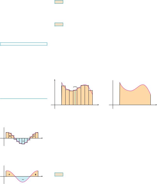
We know that if f happens to be positive, then the Riemann sum can be interpreted as a sum of areas of approximating rectangles (see Figure 1). By comparing Definition 2 with the definition of area in Section 5.1, we see that the definite integral xab f ! x" dx can be interpreted as the area under the curve y ! f ! x" from a to b. (See Figure 2.)
y |
|
|
|
|
|
|
ëx |
|
|
0 |
a |
x*i |
b |
x |
y
y=Ä
0 |
a |
b |
x |
y
y=Ä
0 |
a |
b |
x |
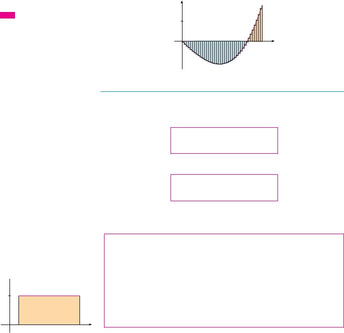
FIGURE 3
µ"f(x*i )"ëx is an approximation to the net area
y
y=Ä
0 a |
b x |
FIGURE 4
jab Ä"dx is the net area
FIGURE 1 |
FIGURE 2 |
If Äù0, the Riemann sum µ"f(xi*)"ëx |
If Äù0, the integral jab Ä"dx is the |
is the sum of areas of rectangles. |
area under the curve y=Ä from a to b. |
If f takes on both positive and negative values, as in Figure 3, then the Riemann sum is the sum of the areas of the rectangles that lie above the x-axis and the negatives of the areas of the rectangles that lie below the x-axis (the areas of the gold rectangles minus the areas of the blue rectangles). When we take the limit of such Riemann sums, we get the situation illustrated in Figure 4. A definite integral can be interpreted as a net area, that is, a difference of areas:
yab f !x" dx ! A1 % A2
where A1 is the area of the region above the x-axis and below the graph of f, and A2 is the area of the region below the x-axis and above the graph of f.
NOTE 4 Although we have defined xab f ! x" dx by dividing )a, b* into subintervals of equal width, there are situations in which it is advantageous to work with subintervals of unequal width. For instance, in Exercise 14 in Section 5.1 NASA provided velocity data at times that were not equally spaced, but we were still able to estimate the distance traveled. And there are methods for numerical integration that take advantage of unequal subintervals.

368 |||| CHAPTER 5 INTEGRALS
If the subinterval widths are (x1, (x2, . . . , (xn, we have to ensure that all these widths approach 0 in the limiting process. This happens if the largest width, max (xi, approaches 0. So in this case the definition of a definite integral becomes
b f ! x" dx ! |
|
n |
lim |
& f ! x*i " (xi |
|
ya |
max (xi l0 |
i!1 |
NOTE 5 We have defined the definite integral for an inegrable function, but not all functions are integrable (see Exercises 67–68). The following theorem shows that the most commonly occurring functions are in fact integrable. It is proved in more advanced courses.
3 |
THEOREM If f is continuous on )a, b*, or if f has only a finite number of |
jump discontinuities, then f is integrable on )a, b*; that is, the definite integral |
|
xab |
f ! x" dx exists. |
If f is integrable on )a, b*, then the limit in Definition 2 exists and gives the same value no matter how we choose the sample points x*i . To simplify the calculation of the integral we often take the sample points to be right endpoints. Then x*i ! xi and the definition of an integral simplifies as follows.
4 |
THEOREM |
If f is integrable on )a, b*, then |
|
|
|||||||
|
|
|
|
|
|
|
|
n |
|
|
|
|
|
|
|
b f ! x" dx ! lim & f !xi" (x |
|
||||||
|
|
ya |
|
|
|
n l' i!1 |
|
|
|||
where |
(x ! |
|
b % a |
|
and |
|
xi ! a " i (x |
|
|||
|
n |
|
|
|
|
|
|||||
|
|
|
|
|
|
|
|
|
|||
EXAMPLE 1 Express |
|
|
|
|
|
|
|
|
|||
|
|
|
|
|
n |
|
|
|
|
|
|
|
|
|
|
lim |
& |
! xi3 |
" xi sin xi" (x |
|
|||
|
|
|
|
n l' |
|
|
|
|
|
||
|
|
|
|
|
i!1 |
|
|
|
|
|
|
as an integral on the interval )0, #*. |
|
|
|
|
|
|
|
||||
SOLUTION |
Comparing the given limit with the limit in Theorem 4, we see that they will |
|
|||||||||
be identical if we choose f !x" ! x3 " x sin x. We are given that a ! 0 and b ! #. |
|
||||||||||
Therefore, by Theorem 4, we have |
|
|
|
|
|
|
|
||||
|
|
n |
|
|
|
|
|
|
# |
|
|
|
|
lim & ! xi3 |
" xi sin xi" (x ! |
|
M |
||||||
|
|
|
!x3 " x sin x" dx |
||||||||
|
|
n l' i!1 |
|
|
|
|
|
y0 |
|
||
Later, when we apply the definite integral to physical situations, it will be important to recognize limits of sums as integrals, as we did in Example 1. When Leibniz chose the notation for an integral, he chose the ingredients as reminders of the limiting process. In general, when we write
n |
b f ! x" dx |
lim & f ! x*i " (x ! |
|
n l' i!1 |
ya |
we replace lim , by x, x*i by x, and (x by dx. |
|

N Formulas 8–11 are proved by writing out each side in expanded form. The left side of Equation 9 is
ca1 " ca2 " & & & " can
The right side is
c!a1 " a2 " & & & " an "
These are equal by the distributive property. The other formulas are discussed in Appendix E.
SECTION 5.2 THE DEFINITE INTEGRAL |||| 369
EVALUATING INTEGRALS
When we use a limit to evaluate a definite integral, we need to know how to work with sums. The following three equations give formulas for sums of powers of positive integers. Equation 5 may be familiar to you from a course in algebra. Equations 6 and 7 were discussed in Section 5.1 and are proved in Appendix E.
|
n |
|
|
n!n " 1" |
|
|
||
5 |
& i ! |
|
|
|||||
|
|
|||||||
|
i!1 |
|
2 |
|
|
|
||
6 |
& i 2 |
! n!n " 1"!2n " 1" |
||||||
|
n |
|
|
|
|
|
|
|
|
i!1 |
|
$ |
|
6 |
% |
||
|
i!1 |
|
|
2 |
|
|||
|
n |
|
|
|
n!n |
" 1" |
2 |
|
7 |
& i 3 ! |
|
|
|
|
|
|
|
The remaining formulas are simple rules for working with sigma notation:
|
|
n |
|
|
8 |
|
& c ! nc |
|
|
|
|
i!1 |
|
|
|
|
n |
|
n |
9 |
|
& cai ! c |
& ai |
|
|
|
i!1 |
i!1 |
|
|
n |
n |
|
n |
10 |
& |
!ai " bi " ! & ai " & bi |
||
|
i!1 |
i!1 |
i!1 |
|
|
n |
n |
|
n |
11 |
& |
!ai % bi " ! & ai % & bi |
||
|
i!1 |
i!1 |
i!1 |
|
EXAMPLE 2
(a)Evaluate the Riemann sum for f !x" ! x3 % 6x taking the sample points to be right endpoints and a ! 0, b ! 3, and n ! 6.
(b)Evaluate y03 ! x3 % 6x" dx.
SOLUTION
(a) With n ! 6 the interval width is
(x ! |
b % a |
! |
3 % 0 |
! |
1 |
n |
6 |
2 |
and the right endpoints are x1 ! 0.5, x2 ! 1.0, x3 ! 1.5, x4 ! 2.0, x5 ! 2.5, and x6 ! 3.0. So the Riemann sum is
6
R6 ! & f ! xi " (x
i!1
!f !0.5" (x " f !1.0" (x " f !1.5" (x " f !2.0" (x " f !2.5" (x " f !3.0" (x
!12 !%2.875 % 5 % 5.625 % 4 " 0.625 " 9"
!%3.9375
370 |
|||| |
CHAPTER 5 INTEGRALS |
|
y |
|
|
|
5 |
|
y=þ-6x |
|
0 |
|
3 |
x |
Notice that f is not a positive function and so the Riemann sum does not represent a sum of areas of rectangles. But it does represent the sum of the areas of the gold rectangles (above the x-axis) minus the sum of the areas of the blue rectangles (below the x-axis) in Figure 5.
(b) With n subintervals we have
b % a 3 (x ! n ! n
FIGURE 5
N In the sum, n is a constant (unlike i), so we can move 3#n in front of the , sign.
y
5y=þ-6x
|
|
AÁ |
|
|
|
|
|
0 |
Aª |
3 x |
|
|
|
|
|
FIGURE 6
j03 (þ-6x)"dx=AÁ-Aª=_6.75
Thus x0 ! 0, x1 ! 3#n, x2 ! 6#n, x3 ! 9#n, and, in general, xi ! 3i#n. Since we are using right endpoints, we can use Theorem 4:
|
n |
n |
|
3i |
|
3 |
|
3 |
! x3 % 6x" dx ! lim & f ! xi " (x ! lim & f |
|
|||||
y0 |
' n |
( n |
|||||
n l' i!1 |
n l' i!1 |
||||||
! lim
n l'
! lim
n l'
! lim
n l'
! lim
n l'
! lim
n l'
81
! 4
n i!1 |
$' n ( |
3 |
|
|
' n (% |
||||||||||
3 |
n |
|
|
3i |
|
|
|
|
3i |
||||||
|
& |
|
|
|
|
|
% 6 |
|
|
% |
|
|
|||
3 |
n |
|
27 |
|
|
18 |
|
|
|
||||||
& |
|
|
i3 |
% |
i |
|
|
||||||||
n |
|
|
3 |
n |
|
|
|
|
|||||||
i!1 |
$ n |
|
|
|
|
|
|
|
|||||||
|
81 |
|
n |
|
|
|
542 |
n |
|
|
% |
|
|||
|
|
& i3 % |
& i |
|
|||||||||||
|
4 |
|
|
||||||||||||
$ n |
i!1 |
|
n |
i!1 |
|
|
|
||||||||
- n4 |
$ |
|
|
2 |
|
% |
|
% n2 2 . |
|||||||
|
81 |
|
|
n!n " 1" |
|
2 |
|
|
|
54 n!n " 1" |
|||||
$814 '1 " 1n (2 % 27'1 " 1n (%
%27 ! % 274 ! %6.75
(Equation 9 with c ! 3#n)
(Equations 11 and 9)
(Equations 7 and 5)
This integral can’t be interpreted as an area because f takes on both positive and negative values. But it can be interpreted as the difference of areas A1 % A2, where A1 and A2 are shown in Figure 6.
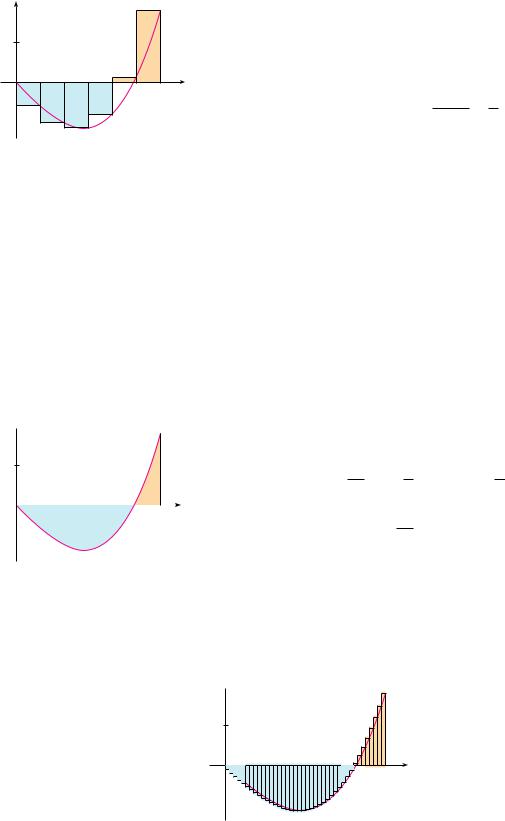
Figure 7 illustrates the calculation by showing the positive and negative terms in the right Riemann sum Rn for n ! 40. The values in the table show the Riemann sums approaching the exact value of the integral, %6.75, as n l '.
FIGURE 7
R¢ü•_6.3998
y
5y=þ-6x
0 |
3 |
x |
n |
Rn |
|
|
40 |
%6.3998 |
100 |
%6.6130 |
500 |
%6.7229 |
1000 |
%6.7365 |
5000 |
%6.7473 |
|
|
M
N Because f ! x" ! e x is positive, the integral in Example 3 represents the area shown in Figure 8.
y
y=«
10
|
|
|
|
|
|
0 |
1 |
3 |
x |
||
FIGURE 8
N A computer algebra system is able to find an explicit expression for this sum because it is a geometric series. The limit could be found using l’Hospital’s Rule.
SECTION 5.2 THE DEFINITE INTEGRAL |||| 371
A much simpler method for evaluating the integral in Example 2 will be given in Section 5.3.
EXAMPLE 3
(a)Set up an expression for x13 ex dx as a limit of sums.
(b)Use a computer algebra system to evaluate the expression.
SOLUTION
(a) Here we have f ! x" ! ex, a ! 1, b ! 3, and
b % a 2 (x ! n ! n
So x0 ! 1, x1 ! 1 " 2#n, x2 ! 1 " 4#n, x3 ! 1 " 6#n, and
2i xi ! 1 " n
From Theorem 4, we get
|
|
n |
|
|
|
|
|
|
|
3 |
ex dx ! lim |
& f ! xi " (x |
|
|
|||||
y1 |
n l' i!1 |
|
|
|
|
|
|
||
|
|
n |
|
|
|
2i |
|
2 |
|
|
! lim |
& f |
|
1 " |
|||||
|
' |
n |
( n |
||||||
|
n l' i!1 |
|
|
||||||
|
|
2 |
|
n |
|
|
|
|
|
|
! lim |
|
|
& |
e1"2i#n |
|
|
||
|
n |
|
|
||||||
|
n l' |
|
|
|
|
||||
|
|
i!1 |
|
|
|
|
|||
(b) If we ask a computer algebra system to evaluate the sum and simplify, we obtain
n |
e!3n"2"#n % e!n"2"#n |
||
& e1"2i#n ! |
|
|
|
e |
2#n |
% 1 |
|
i!1 |
|
||
Now we ask the computer algebra system to evaluate the limit:
|
y |
|
|
y=Пггггг1-≈ |
|
|
|
|
|
|
|||
1 |
|
|
|
|
||
|
|
or |
|
|
||
|
|
|
|
≈+´=1 |
|
|
|
|
|
|
|
|
|
0 |
|
|
1 |
x |
||
FIGURE 9 |
|
|
|
|||
3 |
|
2 |
|
e!3n"2"#n % e!n"2"#n |
|
|
y1 |
ex dx ! lim |
|
! |
|
! e3 |
% e |
|
e2#n % 1 |
|||||
n l' n |
|
|
|
|||
We will learn a much easier method for the evaluation of integrals in the next section. M
V EXAMPLE 4 Evaluate the following integrals by interpreting each in terms of areas.
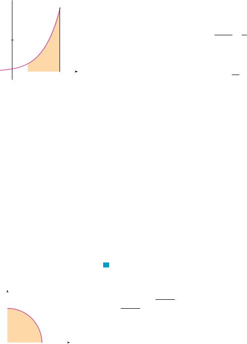
(a) y01 s |
|
dx |
(b) y03 ! x % 1" dx |
1 % x2 |
SOLUTION
(a) Since f !x" ! s1 % x2 + 0, we can interpret this integral as the area under the curve y ! s1 % x2 from 0 to 1. But, since y2 ! 1 % x2, we get x2 " y2 ! 1, which shows that the graph of f is the quarter-circle with radius 1 in Figure 9. Therefore
1 |
|
|
|
# |
|
|
|
||
y0 s1 % x2 |
dx ! 41 |
#!1"2 ! |
|
|
4 |
||||
(In Section 7.3 we will be able to prove that the area of a circle of radius r is #r2.)
372 |||| CHAPTER 5 INTEGRALS
(b) The graph of y ! x % 1 is the line with slope 1 shown in Figure 10. We compute the integral as the difference of the areas of the two triangles:
y03 ! x % 1" dx ! A1 % A2 ! 12 !2 & 2" % 12 !1 & 1" ! 1.5
|
y |
|
|
(3,"2) |
|
|
|
|
|
|
|
||||
|
|
|
|
|
|
||
|
|
|
y=x-1 |
|
|
|
|
|
|
|
|
AÁ |
|
|
|
|
|
|
|
|
|
|
x |
|
0 |
|
Aª 1 |
3 |
|
||
FIGURE 10 |
_1 |
|
|
|
|
|
M |
|
|
|
|
|
|
||
THE MIDPOINT RULE
TEC Module 5.2/7.7 shows how the Midpoint Rule estimates improve as n increases.
y |
1 |
|
|
|
|
|
|
|
y= x |
|
|
0 |
1 |
2 |
x |
FIGURE 11
We often choose the sample point x*i to be the right endpoint of the ith subinterval because it is convenient for computing the limit. But if the purpose is to find an approximation to an integral, it is usually better to choose x*i to be the midpoint of the interval, which we denote by xi. Any Riemann sum is an approximation to an integral, but if we use midpoints we get the following approximation.
MIDPOINT RULE
|
|
|
|
n |
|||||||
b |
f !x" dx / & f ! |
|
i " (x ! (x ) f ! |
|
1" " &&& " f ! |
|
n "* |
||||
x |
x |
x |
|||||||||
ya |
|
|
|
i!1 |
|||||||
where |
(x ! |
b % a |
|
||||||||
n |
|||||||||||
and |
|
|
i ! 21 ! xi%1 " xi " ! midpoint of ) xi%1, xi * |
||||||||
|
x |
||||||||||
V EXAMPLE 5 Use the Midpoint Rule with n ! 5 to approximate y12 1x dx.
SOLUTION The endpoints of the five subintervals are 1, 1.2, 1.4, 1.6, 1.8, and 2.0, so the midpoints are 1.1, 1.3, 1.5, 1.7, and 1.9. The width of the subintervals is (x ! !2 % 1"#5 ! 15 , so the Midpoint Rule gives
y12 1x dx / (x ) f !1.1" " f !1.3" " f !1.5" " f !1.7" " f !1.9"*
! |
1 |
' |
1 |
" |
1 |
" |
1 |
" |
1 |
" |
1 |
( |
5 |
1.1 |
1.3 |
1.5 |
1.7 |
1.9 |
|||||||
/ 0.691908 |
|
|
|
|
|
|
|
|
||||
Since f ! x" ! 1#x $ 0 for 1 ! x ! 2, the integral represents an area, and the approxi- |
|
mation given by the Midpoint Rule is the sum of the areas of the rectangles shown in |
|
Figure 11. |
M |
TEC In Visual 5.2 you can compare left, right, and midpoint approximations to the integral in Example 2 for different values of n.
FIGURE 12
M¢ü•_6.7563
y
cy=c
area=c(b-a)
0 |
a |
b x |
SECTION 5.2 THE DEFINITE INTEGRAL |||| 373
At the moment we don’t know how accurate the approximation in Example 5 is, but in Section 7.7 we will learn a method for estimating the error involved in using the Midpoint Rule. At that time we will discuss other methods for approximating definite integrals.
If we apply the Midpoint Rule to the integral in Example 2, we get the picture in Figure 12. The approximation M40 / %6.7563 is much closer to the true value %6.75 than the right endpoint approximation, R40 / %6.3998, shown in Figure 7.
y |
|
|
5 |
y=þ-6x |
|
0 |
3 |
x |
PROPERTIES OF THE DEFINITE INTEGRAL
When we defined the definite integral xab f ! x" dx, we implicitly assumed that a ) b. But the definition as a limit of Riemann sums makes sense even if a $ b. Notice that if we reverse a and b, then (x changes from !b % a"#n to !a % b"#n. Therefore
yba f ! x" dx ! %yab f ! x" dx
If a ! b, then (x ! 0 and so
yaa f ! x" dx ! 0
We now develop some basic properties of integrals that will help us to evaluate integrals in a simple manner. We assume that f and t are continuous functions.
PROPERTIES OF THE INTEGRAL
1.yab c dx ! c!b % a", where c is any constant
2.yab ) f ! x" " t! x"* dx ! yab f ! x" dx " yab t! x" dx
3. yab cf ! x" dx ! c yab f ! x" dx, where c is any constant
4. yab ) f ! x" % t! x"* dx ! yab f ! x" dx % yab t! x" dx
FIGURE 13 |
Property 1 says that the integral of a constant function f ! x" ! c is the constant times |
|
the length of the interval. If c $ 0 and a ) b, this is to be expected because c!b % a" is |
||
jab c"dx=c(b-a) |
||
the area of the shaded rectangle in Figure 13. |
374 |
|||| |
CHAPTER 5 INTEGRALS |
||
y |
|
|
|
|
|
|
|
f+g |
|
|
|
g |
f |
|
|
|
|
|
|
0 |
a |
|
b |
x |
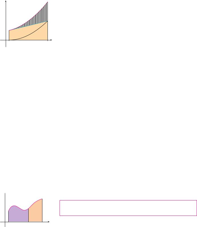
FIGURE 14
jab ![Ä+©]!dx=
jab !Ä!dx+jab !©!dx
N Property 3 seems intuitively reasonable because we know that multiplying a function by a positive number c stretches or shrinks its graph vertically by a factor of c. So it stretches or shrinks each approximating rectangle by a factor c and therefore it has the effect of multiplying the area by c.
y
y=Ä
0 a |
c |
b |
x |
FIGURE 15
Property 2 says that the integral of a sum is the sum of the integrals. For positive functions it says that the area under f # t is the area under f plus the area under t. Figure 14 helps us understand why this is true: In view of how graphical addition works, the corresponding vertical line segments have equal height.
In general, Property 2 follows from Theorem 4 and the fact that the limit of a sum is the sum of the limits:
b & f !x" # t!x"' dx ! lim |
n |
|
|
|
|
|
# & f !xi " # t! xi "' 'x |
|
|
||||
ya |
n l& i!1 |
|
|
|
% |
|
|
|
|
n |
n |
|
|
|
! lim |
|
# f ! xi " 'x # # t! xi " 'x |
|||
|
n l& |
$i!1 |
i!1 |
|
||
|
|
n |
|
n |
t! xi " 'x |
|
|
! lim |
|
f ! xi " 'x # lim |
|||
|
n l& i#!1 |
|
n l& i#!1 |
|
|
|
! yab f ! x" dx # yab t! x" dx
Property 3 can be proved in a similar manner and says that the integral of a constant times a function is the constant times the integral of the function. In other words, a constant (but only a constant) can be taken in front of an integral sign. Property 4 is proved by writing f % t ! f # !%t" and using Properties 2 and 3 with c ! %1.
EXAMPLE 6 Use the properties of integrals to evaluate y01 !4 # 3x2 " dx.
SOLUTION Using Properties 2 and 3 of integrals, we have
y01 !4 # 3x2 " dx ! y01 4 dx # y01 3x2 dx ! y01 4 dx # 3 y01 x2 dx
We know from Property 1 that
y01 4 dx ! 4!1 % 0" ! 4
and we found in Example 2 in Section 5.1 that y01 x2 dx ! 13 . So
y01 !4 # 3x2 " dx ! y01 4 dx # 3 y01 x2 dx
! 4 # 3 |
$ 31 ! 5 |
M |
The next property tells us how to combine integrals of the same function over adjacent intervals:
5.yac f !x" dx # ycb f ! x" dx ! yab f ! x" dx
This is not easy to prove in general, but for the case where f !x" " 0 and a ! c ! b Property 5 can be seen from the geometric interpretation in Figure 15: The area under y ! f ! x" from a to c plus the area from c to b is equal to the total area from a to b.
y |
|
|
|
M |
|
|
|
|
|
y=Ä |
|
m |
|
|
|
0 |
a |
b |
x |
FIGURE 16
|
|
|
|
SECTION 5.2 THE DEFINITE INTEGRAL |
|||| 375 |
|
|
|
|
10 |
8 |
10 |
f ! x" dx. |
V |
|
EXAMPLE 7 If it is known that x0 |
f ! x" dx ! 17 and x0 |
f ! x" dx ! 12, find x8 |
||
SOLUTION |
By Property 5, we have |
|
|
|
||
|
|
|
y08 f ! x" dx # y810 f ! x" dx ! y010 f !x" dx |
|
||
so |
|
y810 f !x" dx ! y010 f ! x" dx % y08 f ! x" dx ! 17 % 12 ! 5 |
M |
|||
Properties 1–5 are true whether a ! b, a ! b, or a ) b. The following properties, in which we compare sizes of functions and sizes of integrals, are true only if a ( b.
COMPARISON PROPERTIES OF THE INTEGRAL
6.If f ! x" " 0 for a ( x ( b, then yab f ! x" dx " 0.
7.If f ! x" " t! x" for a ( x ( b, then yab f !x" dx " yab t!x" dx.
8.If m ( f ! x" ( M for a ( x ( b, then
m!b % a" ( yab f ! x" dx ( M!b % a"
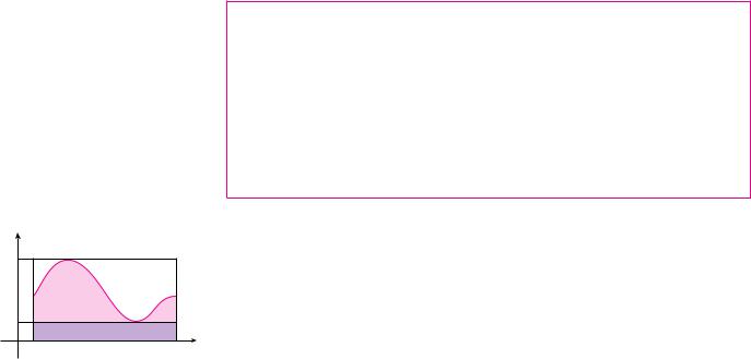
If f ! x" " 0, then xab f !x" dx represents the area under the graph of f, so the geometric interpretation of Property 6 is simply that areas are positive. But the property can be proved from the definition of an integral (Exercise 64). Property 7 says that a bigger function has a bigger integral. It follows from Properties 6 and 4 because f % t " 0.
Property 8 is illustrated by Figure 16 for the case where f !x" " 0. If f is continuous we could take m and M to be the absolute minimum and maximum values of f on the interval &a, b'. In this case Property 8 says that the area under the graph of f is greater than the area of the rectangle with height m and less than the area of the rectangle with height M.
PROOF OF PROPERTY 8 Since m ( f ! x" ( M, Property 7 gives |
|
yab m dx ( yab f ! x" dx ( yab M dx |
|
Using Property 1 to evaluate the integrals on the left and right sides, we obtain |
|
m!b % a" ( yab f !x" dx ( M!b % a" |
M |
Property 8 is useful when all we want is a rough estimate of the size of an integral without going to the bother of using the Midpoint Rule.
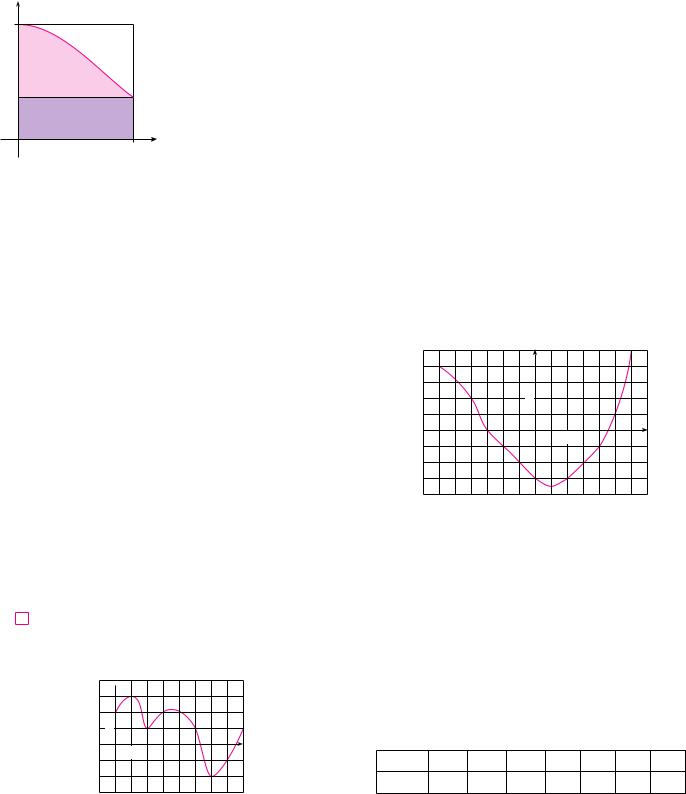
EXAMPLE 8 Use Property 8 to estimate y01 e%x 2 dx.
SOLUTION Because f !x" ! e%x 2 is a decreasing function on &0, 1', its absolute maximum value is M ! f !0" ! 1 and its absolute minimum value is m ! f !1" ! e%1. Thus, by
376 |||| CHAPTER 5 INTEGRALS
y |
y=1 |
|
1 |
|
|
|
|
|
|
y=eÐx2 |
|
|
y=1/e |
|
0 |
1 |
x |
FIGURE 17
Property 8,
|
e%1!1 % 0" ( y01 e%x 2 dx ( 1!1 % 0" |
|
or |
e%1 ( y01 e%x 2 dx ( 1 |
|
|
Since e%1 ( 0.3679, we can write |
|
|
0.367 ( y01 e%x 2 dx ( 1 |
M |
|
The result of Example 8 is illustrated in Figure 17. The integral is greater than the area |
|
of the lower rectangle and less than the area of the square. |
|
|
|
5.2 |
|
EXERCISES |
|
|
|
|
|
|
|
6. The graph of t is shown. Estimate x%3 |
|
t! x" dx with six sub- |
|
1. |
Evaluate the Riemann sum for f ! x" ! 3 % 21 x, 2 ( x ( 14, |
3 |
|||
|
|
with six subintervals, taking the sample points to be left end- |
intervals using (a) right endpoints, (b) left endpoints, and |
|||
|
|
points. Explain, with the aid of a diagram, what the Riemann |
(c) midpoints. |
|
|
|
|
|
sum represents. |
|
|
|
|
2.If f ! x" ! x2 % 2x, 0 ( x ( 3, evaluate the Riemann sum with n ! 6, taking the sample points to be right endpoints. What does the Riemann sum represent? Illustrate with a diagram.
3.If f ! x" ! ex % 2, 0 ( x ( 2, find the Riemann sum with
n ! 4 correct to six decimal places, taking the sample points to be midpoints. What does the Riemann sum represent? Illustrate with a diagram.
4.(a) Find the Riemann sum for f ! x" ! sin x, 0 ( x ( 3*)2, with six terms, taking the sample points to be right endpoints. (Give your answer correct to six decimal places.) Explain what the Riemann sum represents with the aid of a sketch.
(b) Repeat part (a) with midpoints as sample points.
5.The graph of a function f is given. Estimate x08 f ! x" dx using four subintervals with (a) right endpoints, (b) left endpoints, and (c) midpoints.
y
f
1
0 |
1 |
x |
y |
|
|
|
|
g |
1 |
|
|
0 |
1 |
x |
7. A table of values of an increasing function f |
is shown. Use |
||||||||
|
the table to find lower and upper estimates for x025 f ! x" dx. |
||||||||
|
|
|
|
|
|
|
|
|
|
|
x |
0 |
5 |
10 |
15 |
|
20 |
25 |
|
|
|
|
|
|
|
|
|
|
|
|
f ! x" |
%42 |
%37 |
%25 |
%6 |
|
15 |
36 |
|
|
|
|
|
|
|
|
|
|
|
8. The table gives the values of a function obtained from an |
|||||||
experiment. Use them to estimate x39 f ! x" dx using three equal |
|||||||
subintervals with (a) right endpoints, (b) left endpoints, and |
|||||||
(c) midpoints. If the function is known to be an increasing |
|||||||
function, can you say whether your estimates are less than or |
|||||||
greater than the exact value of the integral? |
|
|
|||||
x |
3 |
4 |
5 |
6 |
7 |
8 |
9 |
f ! x" |
%3.4 |
%2.1 |
%0.6 |
0.3 |
0.9 |
1.4 |
1.8 |
9–12 Use the Midpoint Rule with the given value of n to approximate the integral. Round the answer to four decimal places.
9. |
y210 sx3 # 1 dx, |
n ! 4 |
10. |
y0 )2 |
cos4x dx, |
n ! 4 |
||
|
|
|
|
|
|
* |
|
|
11. |
y01 sin! x2" dx, |
n ! 5 |
12. |
y15 x2e%x dx, |
n ! 4 |
|||
|
|
|
|
|
|
|
|
|
CAS 13. If you have a CAS that evaluates midpoint approximations and graphs the corresponding rectangles (use middlesum and middlebox commands in Maple), check the answer to Exercise 11 and illustrate with a graph. Then repeat with
n ! 10 and n ! 20.
14.With a programmable calculator or computer (see the instructions for Exercise 7 in Section 5.1), compute the left and right Riemann sums for the function f ! x" ! sin! x2" on the interval &0, 1' with n ! 100. Explain why these estimates show that
0.306 ! y01 sin! x2" dx ! 0.315
Deduce that the approximation using the Midpoint Rule with n ! 5 in Exercise 11 is accurate to two decimal places.
15. Use a calculator or computer to make a table of values of right Riemann sums Rn for the integral x0* sin x dx with
n ! 5, 10, 50, and 100. What value do these numbers appear to be approaching?
16. Use a calculator or computer to make a table of values of left and right Riemann sums Ln and Rn for the integral
x02 e%x 2 dx with n ! 5, 10, 50, and 100. Between what two numbers must the value of the integral lie? Can you make a similar statement for the integral x%21 e%x 2 dx? Explain.
17–20 Express the limit as a definite integral on the given interval.
|
|
n |
xi ln!1 # xi2" 'x, |
&2, 6' |
||||
17. |
lim |
|
||||||
|
n l& i#!1 |
|
|
|
|
|
|
|
18. |
lim |
n |
cos xi |
'x, |
&*, 2*' |
|||
# |
|
xi |
||||||
|
n l& |
|
|
|
|
|
||
|
|
i!1 |
|
|
|
|
|
|
|
|
n |
|
|
|
|
|
|
19. |
n l& # s |
|
|
|
'x, |
&1, 8] |
||
lim |
i!1 |
|
2x*i |
# ! x*i |
" 2 |
|||
|
|
|
|
|
|
|
|
|
|
|
n |
&4 % 3! xi*"2 # 6! xi*"5' 'x, &0, 2' |
|||||
20. |
lim |
|
||||||
|
n l& i#!1 |
|
|
|
|
|
|
|
21–25 Use the form of the definition of the integral given in Theorem 4 to evaluate the integral.
21. |
y%51 !1 # 3x" dx |
22. |
y14 ! x2 # 2x % 5" dx |
|
|
|
y02 !2 % x2 " dx |
24. |
y05 !1 # 2x3 " dx |
23. |
||||
|
|
|||
25. |
y12 x3 dx |
|
|
|
|
|
|
|
|
SECTION 5.2 THE DEFINITE INTEGRAL |||| 377
26. (a) Find an approximation to the integral x04 ! x2 % 3x" dx using a Riemann sum with right endpoints and n ! 8.
(b) Draw a diagram like Figure 3 to illustrate the approximation in part (a).
(c) Use Theorem 4 to evaluate x04 ! x2 % 3x" dx.
(d) Interpret the integral in part (c) as a difference of areas and illustrate with a diagram like Figure 4.
|
b |
|
|
b2 |
% a2 |
|
|
|
27. |
Prove that ya |
x dx ! |
|
|
|
|
. |
|
|
|
|
2 |
|
||||
|
b |
|
|
|
b |
3 % a |
3 |
|
28. |
Prove that ya |
x2 dx ! |
|
|
|
|
. |
|
|
|
3 |
|
|||||
29–30 Express the integral as a limit of Riemann sums. Do not evaluate the limit.
29. y26 |
x |
dx |
30. y110 ! x % 4 ln x" dx |
1 # x5 |
CAS 31–32 Express the integral as a limit of sums. Then evaluate, using a computer algebra system to find both the sum and the limit.
* |
|
32. y210 x6 dx |
31. y0 |
sin 5x dx |
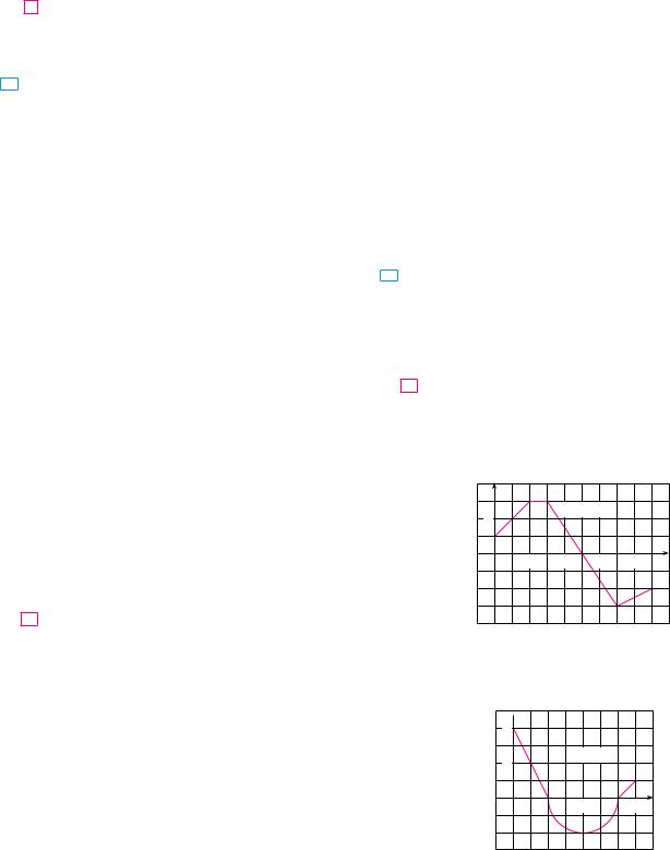
33.The graph of f is shown. Evaluate each integral by interpreting it in terms of areas.
(a) y02 |
f ! x" dx |
|
|
(b) |
y05 |
f ! x" dx |
|
(c) y57 |
f ! x" dx |
|
|
(d) |
y09 |
f ! x" dx |
|
|
y |
|
|
|
|
|
|
|
2 |
|
|
y=Ä |
|
|
|
|
|
|
|
|
|
|
|
|
0 |
2 |
4 |
6 |
|
8 |
x |
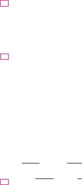
34.The graph of t consists of two straight lines and a semicircle. Use it to evaluate each integral.
(a) y02 t! x" dx |
(b) y26 t! x" dx |
(c) y07 t! x" dx |
y
4
y=©
2
0 |
4 |
7 x |
378 |||| CHAPTER 5 INTEGRALS
35– 40 Evaluate the integral by interpreting it in terms of areas.
35. |
y03 (21 x % 1" dx |
36. |
y%22 |
s |
|
dx |
|||||||||
4 % x2 |
|||||||||||||||
|
|
y%03 (1 # s |
|
) dx |
38. |
y%31 |
!3 % 2x" dx |
||||||||
9 % x2 |
|||||||||||||||
37. |
|||||||||||||||
|
|
||||||||||||||
39. |
y%21 * x * dx |
40. |
y010 * x % 5 * dx |
||||||||||||
|
|
* |
|
|
|
|
|
|
|
|
|
|
|||
41. |
Evaluate y* sin2x cos4x dx. |
|
|
|
|
|
|
||||||||
42. |
Given that y01 3xs |
|
dx ! 5s |
|
% 8, what is |
||||||||||
x2 # 4 |
5 |
||||||||||||||
|
|
y10 3us |
|
|
du? |
|
|
|
|
|
|
||||
|
|
u2 # 4 |
|
|
|
|
|
|
|||||||
43. |
In Example 2 in Section 5.1 we showed that x01 x2 dx ! 31 . |
||||||||||||||
|
|
Use this fact and the properties of integrals to evaluate |
|||||||||||||
|
|
x01 !5 % 6x2 " dx. |
|
|
|
|
|
|
|||||||
44. Use the properties of integrals and the result of Example 3 to evaluate x13 !2ex % 1" dx.
45.Use the result of Example 3 to evaluate x13 ex#2 dx.
46.Use the result of Exercise 27 and the fact that x0*)2 cos x dx ! 1 (from Exercise 25 in Section 5.1), together with the properties of integrals, to evaluate x0*)2 !2 cos x % 5x" dx.
47.Write as a single integral in the form xab f ! x" dx:
y%22 f ! x" dx # y25 f ! x" dx % y%%21 f ! x" dx
48. If x15 f ! x" dx ! 12 and x45 f ! x" dx ! 3.6, find x14 f ! x" dx.
49. If x09 f ! x" dx ! 37 and x09 t! x" dx ! 16, find x09 &2 f ! x" # 3t! x"' dx.
50. Find x05 f ! x" dx if |
|
3 |
for x ! 3 |
f ! x" ! +x |
for x " 3 |
51. Suppose f has absolute minimum value m and absolute maximum value M. Between what two values must x02 f ! x" dx lie? Which property of integrals allows you to make your conclusion?
52–54 Use the properties of integrals to verify the inequality without evaluating the integrals.
52.y01 s1 # x2 dx ( y01 s1 # x dx
53.2 ( y%11 s1 # x2 dx ( 2s2
|
s |
2 |
* |
)4 |
|
s |
3 |
* |
|
|
|
|
|
* |
|
|
|
|
|
54. |
|
( y*)6 |
cos x dx ( |
|
|
|
|
||
24 |
24 |
|
|||||||
55 – 60 Use Property 8 to estimate the value of the integral.
55. |
y14 |
s |
|
dx |
56. |
y02 |
|
1 |
dx |
|
x |
|
|||||||||
|
1 # x2 |
|||||||||
57. |
y*))43 tan x dx |
58. |
y02 |
|
! x3 % 3x # 3" dx |
|||||
|
* |
|
|
|
|
|
|
|
|
|
|
2 |
|
|
|
|
2 |
* |
|
|
|
59. |
y0 |
xe%x dx |
60. |
y* |
|
|
! x % 2 sin x" dx |
|||
61– 62 Use properties of integrals, together with Exercises 27 and 28, to prove the inequality.
3 |
26 |
)2 |
* |
2 |
|
||||
|
|
|
|
|
* |
|
|
|
|
61. y1 |
sx4 # 1 dx " |
|
62. y0 |
x sin x dx ( |
|
|
|||
3 |
8 |
||||||||
63.Prove Property 3 of integrals.
64.Prove Property 6 of integrals.
65. If f is continuous on &a, b', show that
* yab f ! x" dx * ( yab * f ! x" * dx
[Hint: %* f ! x" * ( f ! x" ( * f ! x" *.]
66. Use the result of Exercise 65 to show that
*y02 |
* |
f ! x" sin 2x dx * ( y02 |
* |
* f ! x" * dx |
|
|
|
67.Let f ! x" ! 0 if x is any rational number and f ! x" ! 1 if x is any irrational number. Show that f is not integrable on &0, 1'.
68.Let f !0" ! 0 and f ! x" ! 1)x if 0 ! x ( 1. Show that f is not integrable on &0, 1'. [Hint: Show that the first term in the Riemann sum, f !x*i " 'x, can be made arbitrarily large.]
69– 70 Express the limit as a definite integral.
69. |
lim |
n |
i 4 |
|
[Hint: Consider f ! x" ! x4.] |
|||||||||||
|
|
n5 |
||||||||||||||
|
n l& i#!1 |
|
|
|
|
|
|
|
|
|
|
|||||
70. |
lim |
1 |
|
n |
|
1 |
|
|
|
|
|
|
|
|
||
n i#!1 1 # !i)n"2 |
|
|
|
|
|
|
|
|||||||||
|
n l& |
|
|
|
|
|
|
|
||||||||
71. |
Find x12 x%2 dx. Hint: Choose xi* to be the geometric mean of |
|||||||||||||||
|
xi%1 and xi |
(that is, xi* ! s |
xi%1 xi |
) and use the identity |
||||||||||||
|
|
|
|
|
|
|
1 |
1 |
1 |
|
||||||
|
|
|
|
|
|
|
|
|
|
! |
|
% |
|
|
||
|
|
|
|
|
|
|
|
m!m # 1" |
m |
m # 1 |
||||||