INTEGRALS

5.1

N Now is a good time to read (or reread)

A Preview of Calculus (see page 2). It discusses the unifying ideas of calculus and helps put in perspective where we have been and where we are going.

FIGURE 1

S=s(x,!y)!|!aøxøb, 0øyøÄd

AREAS AND DISTANCES

In this section we discover that in trying to find the area under a curve or the distance traveled by a car, we end up with the same special type of limit.

THE AREA PROBLEM

We begin by attempting to solve the area problem: Find the area of the region S that lies under the curve y ! f !x" from a to b. This means that S, illustrated in Figure 1, is bounded by the graph of a continuous function f [where f !x" ! 0], the vertical lines x ! a and x ! b, and the x-axis.

y

y=Ä

x=a

S x=b

y

(1,!1)

y=≈

S

FIGURE 3

However, it isn’t so easy to find the area of a region with curved sides. We all have an intuitive idea of what the area of a region is. But part of the area problem is to make this intuitive idea precise by giving an exact definition of area.

Recall that in defining a tangent we first approximated the slope of the tangent line by slopes of secant lines and then we took the limit of these approximations. We pursue a similar idea for areas. We first approximate the region S by rectangles and then we take the limit of the areas of these rectangles as we increase the number of rectangles. The following example illustrates the procedure.

V EXAMPLE 1 Use rectangles to estimate the area under the parabola y ! x2 from 0 to 1 (the parabolic region S illustrated in Figure 3).

SOLUTION We first notice that the area of S must be somewhere between 0 and 1 because S is contained in a square with side length 1, but we can certainly do better than that.

y

(1,!1)

y=≈

We can approximate each strip by a rectangle whose base is the same as the strip and whose height is the same as the right edge of the strip [see Figure 4(b)]. In other words, the heights of these rectangles are the values of the function f !x" ! x2 at the right endpoints of the subintervals [0, 14 ], [14 , 12 ], [12 , 34 ], and [34 , 1].

Each rectangle has width 14 and the heights are (14 )2, (12 )2, (34 )2, and 12. If we let R4 be the sum of the areas of these approximating rectangles, we get

R4 ! 14 ! (14 )2 # 14 ! (12 )2 # 14 ! (34 )2 # 14 ! 12 ! 1532 ! 0.46875

From Figure 4(b) we see that the area A of S is less than R4, so

A " 0.46875

Instead of using the rectangles in Figure 4(b) we could use the smaller rectangles in Figure 5 whose heights are the values of f at the left endpoints of the subintervals. (The leftmost rectangle has collapsed because its height is 0.) The sum of the areas of these approximating rectangles is

L4 ! 14 ! 02 # 14 ! (14 )2 # 14 ! (12 )2 # 14 ! (34 )2 ! 327 ! 0.21875

We see that the area of S is larger than L4, so we have lower and upper estimates for A:

0.21875 " A " 0.46875

FIGURE 6

Approximating S with eight rectangles

(a) Using left endpoints

(b) Using right endpoints

SECTION 5.1 AREAS AND DISTANCES |||| 357

By computing the sum of the areas of the smaller rectangles !L8 " and the sum of the areas of the larger rectangles !R8 ", we obtain better lower and upper estimates for A:

0.2734375 " A " 0.3984375

So one possible answer to the question is to say that the true area of S lies somewhere between 0.2734375 and 0.3984375.

We could obtain better estimates by increasing the number of strips. The table at the left shows the results of similar calculations (with a computer) using n rectangles whose heights are found with left endpoints !Ln " or right endpoints !Rn ". In particular, we see by using 50 strips that the area lies between 0.3234 and 0.3434. With 1000 strips we narrow it down even more: A lies between 0.3328335 and 0.3338335. A good estimate is obtained by averaging these numbers: A & 0.3333335. M

From the values in the table in Example 1, it looks as if Rn is approaching 13 as n increases. We confirm this in the next example.

V EXAMPLE 2 For the region S in Example 1, show that the sum of the areas of the upper approximating rectangles approaches 13 , that is,

N Here we are computing the limit of the sequence 'Rn (. Sequences were discussed in

A Preview of Calculus and will be studied in detail in Chapter 11. Their limits are calculated in the same way as limits at infinity (Section 2.6). In particular, we know that

lim 1 ! 0

n l$ n

Perhaps you have seen this formula before. It is proved in Example 5 in Appendix E. Putting Formula 1 into our expression for Rn, we get

TEC In Visual 5.1 you can create pictures like those in Figures 8 and 9 for other values of n.

From Figures 8 and 9 it appears that, as n increases, both Ln and Rn become better and better approximations to the area of S. Therefore, we define the area A to be the limit of the sums of the areas of the approximating rectangles, that is,

A ! lim Rn ! lim Ln ! 13

n l$ n l$

FIGURE 8

y

n=30 R£ü•0.3502

y

n=50 R∞ü=0.3434

y

n=50 L∞ü=0.3234

FIGURE 9

The area is the number that is smaller than all upper sums and larger than all lower sums

FIGURE 10

Let’s apply the idea of Examples 1 and 2 to the more general region S of Figure 1. We start by subdividing S into n strips S1, S2, . . . , Sn of equal width as in Figure 10.

y

y=Ä

y

(a) n=2

FIGURE 12

(b) n=4

(c) n=8

(d) n=12

This tells us to end with i=n.

n

This tells us µ f(xi)!ëx to add.

i=m

This tells us to start with i=m.

N If you need practice with sigma notation, look at the examples and try some of the exercises in Appendix E.

y

1y=eШ

FIGURE 14

It is difficult to evaluate this limit directly by hand, but with the aid of a computer algebra system it isn’t hard (see Exercise 24). In Section 5.3 we will be able to find A more easily using a different method.

(b) With n ! 4 the subintervals of equal width &x ! 0.5 are )0, 0.5*, )0.5, 1*, )1, 1.5*, and )1.5, 2*. The midpoints of these subintervals are x1* ! 0.25, x2* ! 0.75, x3* ! 1.25, and x4* ! 1.75, and the sum of the areas of the four approximating rectangles (see Figure 14) is

4

M4 ! + f !x*i " &x

i!1

!f !0.25" &x # f !0.75" &x # f !1.25" &x # f !1.75" &x

!e'0.25!0.5" # e'0.75!0.5" # e'1.25!0.5" # e'1.75!0.5"

!12 !e'0.25 # e'0.75 # e'1.25 # e'1.75 " & 0.8557

So an estimate for the area is

A & 0.8557

FIGURE 15

With n ! 10 the subintervals are )0, 0.2*, )0.2, 0.4*, . . . , )1.8, 2* and the midpoints are x1* ! 0.1, x2* ! 0.3, x3* ! 0.5, . . . , x10* ! 1.9. Thus

A& M10 ! f !0.1" &x # f !0.3" &x # f !0.5" &x # %%% # f !1.9" &x

! 0.2!e'0.1 # e'0.3 # e'0.5 # %%% # e'1.9 " & 0.8632

THE DISTANCE PROBLEM

Now let’s consider the distance problem: Find the distance traveled by an object during a certain time period if the velocity of the object is known at all times. (In a sense this is the inverse problem of the velocity problem that we discussed in Section 2.1.) If the velocity remains constant, then the distance problem is easy to solve by means of the formula

distance ! velocity ( time

But if the velocity varies, it’s not so easy to find the distance traveled. We investigate the problem in the following example.

V EXAMPLE 4 Suppose the odometer on our car is broken and we want to estimate the distance driven over a 30-second time interval. We take speedometer readings every five seconds and record them in the following table:

In order to have the time and the velocity in consistent units, let’s convert the velocity readings to feet per second (1 mi%h ! 5280%3600 ft%s):

During the first five seconds the velocity doesn’t change very much, so we can estimate the distance traveled during that time by assuming that the velocity is constant. If we take the velocity during that time interval to be the initial velocity (25 ft%s), then we obtain the approximate distance traveled during the first five seconds:

25 ft%s ( 5 s ! 125 ft

Similarly, during the second time interval the velocity is approximately constant and we take it to be the velocity when t ! 5 s. So our estimate for the distance traveled from

t ! 5 s to t ! 10 s is

31 ft%s ( 5 s ! 155 ft

If we add similar estimates for the other time intervals, we obtain an estimate for the total distance traveled:

!25 ( 5" # !31 ( 5" # !35 ( 5" # !43 ( 5" # !47 ( 5" # !46 ( 5" ! 1135 ft

FIGURE 16

SECTION 5.1 AREAS AND DISTANCES |||| 363

We could just as well have used the velocity at the end of each time period instead of the velocity at the beginning as our assumed constant velocity. Then our estimate becomes

!31 ( 5" # !35 ( 5" # !43 ( 5" # !47 ( 5" # !46 ( 5" # !41 ( 5" ! 1215 ft

If we had wanted a more accurate estimate, we could have taken velocity readings every two seconds, or even every second. M

Perhaps the calculations in Example 4 remind you of the sums we used earlier to estimate areas. The similarity is explained when we sketch a graph of the velocity function of the car in Figure 16 and draw rectangles whose heights are the initial velocities for each time interval. The area of the first rectangle is 25 ( 5 ! 125, which is also our estimate for the distance traveled in the first five seconds. In fact, the area of each rectangle can be interpreted as a distance because the height represents velocity and the width represents time. The sum of the areas of the rectangles in Figure 16 is L6 ! 1135, which is our initial estimate for the total distance traveled.

In general, suppose an object moves with velocity v ! f !t", where a ) t ) b and f !t" ! 0 (so the object always moves in the positive direction). We take velocity readings at times t0 !! a", t1, t2, . . . , tn !! b" so that the velocity is approximately constant on each subinterval. If these times are equally spaced, then the time between consecutive readings is &t ! !b ' a"%n. During the first time interval the velocity is approximately f !t0 " and so the distance traveled is approximately f !t0 " &t. Similarly, the distance traveled during the second time interval is about f !t1" &t and the total distance traveled during the time interval )a, b* is approximately

n

f !t0 " &t # f !t1" &t # %%% # f !tn'1" &t ! + f !ti'1" &t

i!1

If we use the velocity at right endpoints instead of left endpoints, our estimate for the total distance becomes

n

f !t1" &t # f !t2 " &t # %%% # f !tn " &t ! + f !ti " &t

i!1

The more frequently we measure the velocity, the more accurate our estimates become, so it seems plausible that the exact distance d traveled is the limit of such expressions:

We will see in Section 5.4 that this is indeed true.

Because Equation 5 has the same form as our expressions for area in Equations 2 and 3, it follows that the distance traveled is equal to the area under the graph of the velocity function. In Chapters 6 and 8 we will see that other quantities of interest in the natural and social sciences—such as the work done by a variable force or the cardiac output of the heart—can also be interpreted as the area under a curve. So when we compute areas in this chapter, bear in mind that they can be interpreted in a variety of practical ways.

5.1EXERCISES

1.(a) By reading values from the given graph of f, use five rectangles to find a lower estimate and an upper estimate for the area under the given graph of f from x ! 0 to

x ! 10. In each case sketch the rectangles that you use.

(b)Find new estimates using ten rectangles in each case.

y

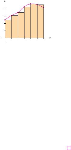
2.(a) Use six rectangles to find estimates of each type for the area under the given graph of f from x ! 0 to x ! 12.

(i)L6 (sample points are left endpoints)

(ii)R6 (sample points are right endpoints)

(iii)M6 (sample points are midpoints)

(b)Is L6 an underestimate or overestimate of the true area?

(c)Is R6 an underestimate or overestimate of the true area?

(d)Which of the numbers L6, R6, or M6 gives the best estimate? Explain.

y

8

y=Ä

4

3.(a) Estimate the area under the graph of f ! x" ! cos x from

x! 0 to x ! ##2 using four approximating rectangles and right endpoints. Sketch the graph and the rectangles. Is your estimate an underestimate or an overestimate?

(b)Repeat part (a) using left endpoints.

4.(a) Estimate the area under the graph of f ! x" ! sx from

x! 0 to x ! 4 using four approximating rectangles and right endpoints. Sketch the graph and the rectangles. Is your estimate an underestimate or an overestimate?

(b)Repeat part (a) using left endpoints.

5. (a) Estimate the area under the graph of f ! x" ! 1 " x2 from x ! %1 to x ! 2 using three rectangles and right end-

points. Then improve your estimate by using six rectangles. Sketch the curve and the approximating rectangles.

(b)Repeat part (a) using left endpoints.

(c)Repeat part (a) using midpoints.

(d)From your sketches in parts (a)–(c), which appears to be the best estimate?

;6. (a) Graph the function f ! x" ! e%x 2, %2 ! x ! 2.

(b)Estimate the area under the graph of f using four approximating rectangles and taking the sample points to be

(i) right endpoints and (ii) midpoints. In each case sketch the curve and the rectangles.

(c)Improve your estimates in part (b) by using 8 rectangles.

7–8 With a programmable calculator (or a computer), it is possible to evaluate the expressions for the sums of areas of approximating rectangles, even for large values of n, using looping. (On a TI use the Is$ command or a For-EndFor loop, on a Casio use Isz, on an HP or in BASIC use a FOR-NEXT loop.) Compute the sum of the areas of approximating rectangles using equal subintervals and right endpoints for n ! 10, 30, 50, and 100. Then guess the value of the exact area.

CAS 9. Some computer algebra systems have commands that will draw approximating rectangles and evaluate the sums of their areas, at least if x*i is a left or right endpoint. (For instance, in Maple use leftbox, rightbox, leftsum, and rightsum.)

(a)If f ! x" ! 1#! x2 " 1", 0 ! x ! 1, find the left and right sums for n ! 10, 30, and 50.

(b)Illustrate by graphing the rectangles in part (a).

(c)Show that the exact area under f lies between 0.780 and 0.791.

CAS 10. (a) If f ! x" ! ln x, 1 ! x ! 4, use the commands discussed in Exercise 9 to find the left and right sums for n ! 10, 30, and 50.

(b)Illustrate by graphing the rectangles in part (a).

(c)Show that the exact area under f lies between 2.50 and 2.59.

11.The speed of a runner increased steadily during the first three seconds of a race. Her speed at half-second intervals is given in the table. Find lower and upper estimates for the distance that she traveled during these three seconds.

12. Speedometer readings for a motorcycle at 12-second intervals are given in the table.

(a) Estimate the distance traveled by the motorcycle during this time period using the velocities at the beginning of the time intervals.

(b) Give another estimate using the velocities at the end of the time periods.

(c) Are your estimates in parts (a) and (b) upper and lower estimates? Explain.

13. Oil leaked from a tank at a rate of r! t" liters per hour. The rate decreased as time passed and values of the rate at twohour time intervals are shown in the table. Find lower and upper estimates for the total amount of oil that leaked out.

14. When we estimate distances from velocity data, it is sometimes necessary to use times t0, t1, t2, t3, . . . that are not equally spaced. We can still estimate distances using the time periods (ti ! ti % ti%1. For example, on May 7, 1992, the space shuttle Endeavour was launched on mission STS-49, the purpose of which was to install a new perigee kick motor in an Intelsat communications satellite. The table, provided by NASA, gives the velocity data for the shuttle between liftoff and the jettisoning of the solid rocket boosters. Use these data to estimate the height above the earth’s surface of the Endeavour, 62 seconds after liftoff.

15.The velocity graph of a braking car is shown. Use it to estimate the distance traveled by the car while the brakes are applied.

√

(ft/s)

60

40

20

16.The velocity graph of a car accelerating from rest to a speed of 120 km#h over a period of 30 seconds is shown. Estimate the distance traveled during this period.

17–19 Use Definition 2 to find an expression for the area under the graph of f as a limit. Do not evaluate the limit.

17.f ! x" ! s4 x , 1 ! x ! 16

18.f ! x" ! lnxx , 3 ! x ! 10

19. f ! x" ! x cos x, 0 ! x ! ## 2

20–21 Determine a region whose area is equal to the given limit. Do not evaluate the limit.

22.(a) Use Definition 2 to find an expression for the area under the curve y ! x3 from 0 to 1 as a limit.

(b)The following formula for the sum of the cubes of the first n integers is proved in Appendix E. Use it to evaluate the limit in part (a).

13 " 23 " 33 " & & & " n3 ! $n!n " 1" %2

2

CAS 23. (a) Express the area under the curve y ! x5 from 0 to 2 as

a limit.

(b)Use a computer algebra system to find the sum in your expression from part (a).

(c)Evaluate the limit in part (a).

CAS 24. Find the exact area of the region under the graph of y ! e%x from 0 to 2 by using a computer algebra system to evaluate the sum and then the limit in Example 3(a). Compare your answer with the estimate obtained in Example 3(b).