Добавил:
Опубликованный материал нарушает ваши авторские права? Сообщите нам.
Вуз: Предмет: Файл:
[James_Stewart]_Single_Variable_Calculus_Early_Tr(BookFi).pdf
Скачиваний:
36
Добавлен:
30.12.2019
Размер:
18.09 Mб
Скачать

FIGURE 1

TEC Visual 8.1 shows an animation

of Figure 2.

8.1ARC LENGTH

What do we mean by the length of a curve? We might think of fitting a piece of string to the curve in Figure 1 and then measuring the string against a ruler. But that might be difficult to do with much accuracy if we have a complicated curve. We need a precise definition for the length of an arc of a curve, in the same spirit as the definitions we developed for the concepts of area and volume.

If the curve is a polygon, we can easily find its length; we just add the lengths of the line segments that form the polygon. (We can use the distance formula to find the distance between the endpoints of each segment.) We are going to define the length of a general curve by first approximating it by a polygon and then taking a limit as the number of segments of the polygon is increased. This process is familiar for the case of a circle, where the circumference is the limit of lengths of inscribed polygons (see Figure 2).

Now suppose that a curve C is defined by the equation y f x , where f is continuous and a x b. We obtain a polygonal approximation to C by dividing the interval a, b into n subintervals with endpoints x0, x1, . . . , xn and equal width x. If yi f xi , then the point Pi xi, yi lies on C and the polygon with vertices P0, P1, . . . , Pn, illustrated in Figure 3, is an approximation to C.


y


P™


y=ƒ


Pi-1


Pi

Pn


FIGURE 2


0 a x¡ ¤

xi-1 xi

b x


FIGURE 3


Pi

Pi

Pi-1

Pi

Pi-1

Pi

Pi-1

Pi-1

FIGURE 4

The length L of C is approximately the length of this polygon and the approximation gets better as we let n increase. (See Figure 4, where the arc of the curve between Pi 1 and Pi has been magnified and approximations with successively smaller values of x are shown.) Therefore we define the length L of the curve C with equation y f x , a x b, as the limit of the lengths of these inscribed polygons (if the limit exists):

n

1 L lim Pi 1Pi

n l i 1

Notice that the procedure for defining arc length is very similar to the procedure we used for defining area and volume: We divided the curve into a large number of small parts. We then found the approximate lengths of the small parts and added them. Finally, we took the limit as n l .

The definition of arc length given by Equation 1 is not very convenient for computational purposes, but we can derive an integral formula for L in the case where f has a continuous derivative. [Such a function f is called smooth because a small change in x produces a small change in f x .]

If we let yi yi yi 1, then

Pi 1Pi s xi xi 1 2 yi yi 1 2 s x 2 yi 2

525

526 |||| CHAPTER 8 FURTHER APPLICATIONS OF INTEGRATION

By applying the Mean Value Theorem to f on the interval xi 1, xi , we find that there is a number xi* between xi 1 and xi such that


f xi f xi 1 f xi* xi xi 1


that is,


yi f xi* x


Thus we have


Pi 1Pi s


s


x 2 yi 2

x 2 f xi* x 2


s


s


s


x


1 [ f xi* 2

x 2


1 f xi* 2

(since x 0)

Therefore, by Definition 1,


n l

n


n


n l s


L lim


Pi 1Pi


lim


1 f xi* 2

x


i 1


i 1


We recognize this expression as being equal to


b


ya s1

f x 2 dx


by the definition of

a definite

integral. This

integral exists

because the function

t x s1 f x 2

is continuous. Thus we have proved the following theorem:


2 THE ARC LENGTH FORMULA


If f is continuous on a, b , then the length of

the curve y f x , a x b, is


b


L ya


s1 f x 2 dx


y

(4,8)

¥=˛

(1,1)

0x

FIGURE 5

If we use Leibniz notation for derivatives, we can write the arc length formula as follows:


y


dy


2


3

L

b

1


dx


a


dx


EXAMPLE 1 Find the length of the arc of the semicubical parabola y2 x3 between the points 1, 1 and 4, 8 . (See Figure 5.)

SOLUTION For the top half of the curve we have


y x3 2

dy

23 x1 2


dx

and so the arc length formula gives

y


4


dy

2

4


L 1


1


dx


dx y1 s1

49 x dx

If we substitute u 1 94 x, then du 94 dx. When x 1, u 134 ; when x 4, u 10.

N As a check on our answer to Example 1, notice from Figure 5 that the arc length ought to be slightly larger than the distance from 1, 1 to4, 8 , which is

s58 7.615773

According to our calculation in Example 1, we have

L 271 (80 s10 13 s13 ) 7.633705

Sure enough, this is a bit greater than the length of the line segment.

N Figure 6 shows the arc of the parabola whose length is computed in Example 2, together with polygonal approximations having n 1 and

n 2 line segments, respectively. For n 1 the approximate length is L1 s2 , the diagonal of a square. The table shows the approximations Ln that we get by dividing 0, 1 into n equal subintervals. Notice that each time we double the number of sides of the polygon, we get closer to the exact length, which is

L s5 ln(s5 2) 1.478943 2 4


SECTION 8.1 ARC LENGTH ||||

527

Therefore


10


10


L 94

y13 4 su du

94

32 u3 2]13 4


8

[103 2 (134 )3 2 ]

1

(80s


13s


)


10

13

M

27

27

If a curve has the equation x t y , c y d, and t y is continuous, then by interchanging the roles of x and y in Formula 2 or Equation 3, we obtain the following formula for its length:


y


dx


2


d


d


4

L yc

s1 t y 2 dy c


1


dy


dy

V EXAMPLE 2 Find the length of the arc of the parabola y2 x from 0, 0 to 1, 1 .

SOLUTION Since x y2, we have dx dy 2y, and Formula 4 gives

y


dx


2


1


1


L 0


1


dy


dy y0 s1

4y2 dy

We make the trigonometric substitution y 12 tan , which gives dy 12 sec2 d and s1 4y2 s1 tan2 sec . When y 0, tan 0, so 0; when y 1,

tan 2, so

tan 1 2 , say. Thus


L y0

sec 21 sec2 d 21 y0 sec3 d


21 21 [sec tan ln sec

tan ]0

(from Example 8 in Section 7.2)

41 (sec tan ln sec

tan )


(We could have used Formula 21 in the Table of Integrals.) Since tan 2, we have


sec2 1 tan2 5, so sec

s5 and


L

s


ln(s


2)


5

5


M


4


2


y


1


n

Ln


x=¥


1

1.414


2

1.445


4

1.464


8

1.472


16

1.476


32

1.478


0


1 x


64

1.479


FIGURE 6

528 |||| CHAPTER 8 FURTHER APPLICATIONS OF INTEGRATION

N Checking the value of the definite integral with a more accurate approximation produced by a computer algebra system, we see that the approximation using Simpson’s Rule is accurate to four decimal places.

Because of the presence of the square root sign in Formulas 2 and 4, the calculation of an arc length often leads to an integral that is very difficult or even impossible to evaluate explicitly. Thus we sometimes have to be content with finding an approximation to the length of a curve, as in the following example.

V EXAMPLE 3

(a)Set up an integral for the length of the arc of the hyperbola xy 1 from the point 1, 1 to the point (2, 12 ).

(b)Use Simpson’s Rule with n 10 to estimate the arc length.

SOLUTION

(a) We have


1


dy

1


y


x


dx

x2


and so the arc length is


y


y


y

s


2


dy

2

2


1


2

x4 1

L 1

1


dx 1

1


dx 1


dx


dx


x4


x2

(b) Using Simpson’s Rule (see Section 7.7) with a 1, b 2, n 10, x 0.1, and f x s1 1 x4 , we have


2

1

1


y


L

x4 dx

1


x

f 1 4 f 1.1 2 f 1.2 4 f 1.3 2 f 1.8 4 f 1.9 f 2


3


1.1321


M

THE ARC LENGTH FUNCTION

We will find it useful to have a function that measures the arc length of a curve from a particular starting point to any other point on the curve. Thus if a smooth curve C has the equation y f x , a x b, let s x be the distance along C from the initial point P0 a, f a to the point Q x, f x . Then s is a function, called the arc length function, and, by Formula 2,


x


5

s x ya s1

f t 2 dt

(We have replaced the variable of integration by t so that x does not have two meanings.) We can use Part 1 of the Fundamental Theorem of Calculus to differentiate Equation 5 (since the integrand is continuous):


ds


dy

2

6


1 f x 2


1


dx

s

dx


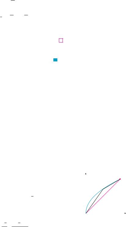
SECTION 8.1 ARC LENGTH |||| 529


Equation 6 shows that the rate of change of s with respect to x is always at least 1 and is


equal to 1 when f x , the slope of the curve, is 0. The differential of arc length is


dx


7


ds

1


dy

2


dx


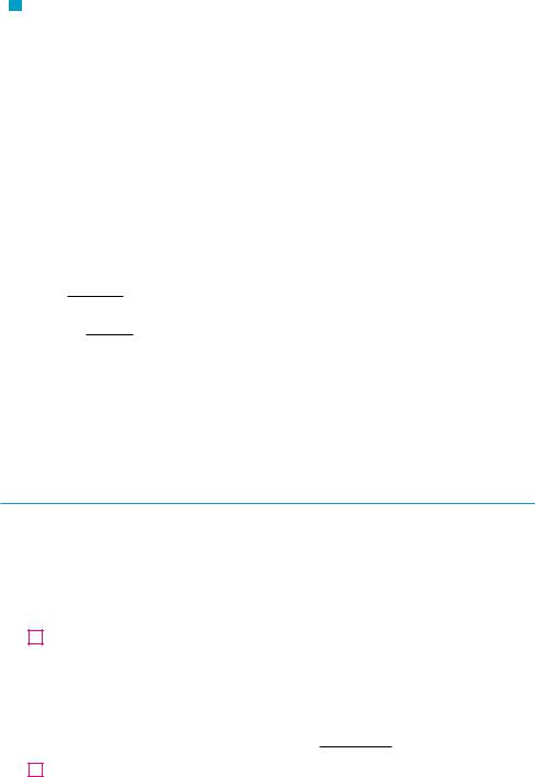
and this equation is sometimes written in the symmetric form


y


8


ds 2 dx 2 dy 2


ds


The geometric interpretation of Equation 8 is shown in Figure 7. It can be used as a


dy


mnemonic device for remembering both of the Formulas 3 and 4. If we write L xds, then


Îs


Îy


dx


from Equation 8 either we can solve to get (7), which gives (3), or we can solve to get


ds

1


dx

2


dy


dy


0


x


FIGURE 7


which gives (4).


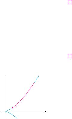
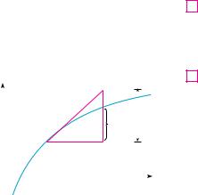
EXAMPLE 4 Find the arc length function for the curve y x2 81 ln x taking P0 1, 1


V


as the starting point.


SOLUTION

If f x x2 81 ln x, then


f x 2x


1


8x


1 f x 2 1


1


2


1


1


2x


1 4x2


64x2


8x


2


1


1


1


2


4x2


2x


2

64x2

8x


s


2x

1


1 f x 2


8x


Thus the arc length function is given by


x


s x y1

s1 f t 2 dt


1

2t 81t dt t2 81 ln t]1


y

x


x


x2 81 ln x 1


For instance, the arc length along the curve from 1, 1 to 3, f 3 is


s 3 32 81 ln 3 1 8

ln 3

8.1373


M


8


530 |||| CHAPTER 8 FURTHER APPLICATIONS OF INTEGRATION


y


y


s(x)


1


N Figure 8 shows the interpretation of the arc

1


length function in Example 4 . Figure 9 shows the


0


1

x


graph of this arc length function. Why is s x


y=≈-1 ln x


negative when x is less than 1?


8


s(x)=≈+1

ln x-1


0


x


1 x


8


FIGURE 8


FIGURE 9


8.1E X E R C I S E S

1.Use the arc length formula (3) to find the length of the curve y 2x 5, 1 x 3. Check your answer by noting that the curve is a line segment and calculating its length by the distance formula.

2.Use the arc length formula to find the length of the curve

y s2 x 2 , 0 x 1. Check your answer by noting that the curve is part of a circle.

3–6 Set up, but do not evaluate, an integral for the length of the curve.

3.

y cos x,

0 x 2

4.

y xe x2, 0 x 1

5.

x y y 3, 1 y 4

6.


x 2


y 2

1


a 2

b 2


7–18 Find the length of the curve.

7.

y 1 6x 3 2, 0 x 1

8.

y 2 4 x 4 3, 0 x 2, y 0

9.

y

x 5


1


, 1 x 2

6


10x 3

10.

x

y 4


1

,

1

y 2

8


4y 2

11.

x

31 s


y 3 ,

1 y 9

y

12.

y ln cos x ,

0 x 3

13.

y ln sec x ,

0 x 4

14. y

3 21 cosh 2x,

0 x 1

15. y ln 1 x 2 , 0 x 12

16.y sx x 2 sin 1(sx )

17.y e x, 0 x 1


e x 1


18. y ln


e x 1


, a x b, a 0


;19–20 Find the length of the arc of the curve from point P to point Q.

19.

y 21 x 2, P( 1, 21 ), Q

(1, 21 )

20.

x 2 y 4 3, P 1, 5 ,

Q 8, 8


;21–22 Graph the curve and visually estimate its length. Then find its exact length.

21.

y 32 x 2 1 3 2,


1 x 3

22.

y

x 3


1

,

1

x 1


2

6


2x


23–26 Use Simpson’s Rule with n 10 to estimate the arc length of the curve. Compare your answer with the value of the integral produced by your calculator.

23.

y xe x, 0

x 5

24.

x y s


,

1 y 2

y

25.

y sec x, 0 x 3

26.

y x ln x, 1 x 3


;27. (a) Graph the curve y x s3 4 x , 0 x 4.

(b)Compute the lengths of inscribed polygons with n 1, 2, and 4 sides. (Divide the interval into equal subintervals.) Illustrate by sketching these polygons (as in Figure 6).

(c)Set up an integral for the length of the curve.

(d)Use your calculator to find the length of the curve to four decimal places. Compare with the approximations in part (b).

;28. Repeat Exercise 27 for the curve

y x sin x 0 x 2

CAS 29. Use either a computer algebra system or a table of integrals to find the exact length of the arc of the curve y ln x that lies between the points 1, 0 and 2, ln 2 .

CAS 30. Use either a computer algebra system or a table of integrals to find the exact length of the arc of the curve y x 4 3 that lies between the points 0, 0 and 1, 1 . If your CAS has trouble evaluating the integral, make a substitution that changes the integral into one that the CAS can evaluate.

31.Sketch the curve with equation x 2 3 y 2 3 1 and use symmetry to find its length.

32.(a) Sketch the curve y 3 x 2.

(b)Use Formulas 3 and 4 to set up two integrals for the arc length from 0, 0 to 1, 1 . Observe that one of these is an improper integral and evaluate both of them.

(c)Find the length of the arc of this curve from 1, 1 to 8, 4 .

33.Find the arc length function for the curve y 2x 3 2 with starting point P0 1, 2 .

;34. (a) Graph the curve y 13 x 3 1 4x , x 0.

(b)Find the arc length function for this curve with starting point P0(1, 127 ).

(c)Graph the arc length function.

35.Find the arc length function for the curve

y sin 1 x s1 x 2 with starting point 0, 1 .

36.A steady wind blows a kite due west. The kite’s height above

ground from horizontal position x 0 to x 80 ft is given by y 150 401 x 50 2. Find the distance traveled by the kite.

37.A hawk flying at 15 m s at an altitude of 180 m accidentally drops its prey. The parabolic trajectory of the falling prey is described by the equation

y 180 x 2 45

until it hits the ground, where y is its height above the ground and x is the horizontal distance traveled in meters. Calculate

SECTION 8.1 ARC LENGTH |||| 531

the distance traveled by the prey from the time it is dropped until the time it hits the ground. Express your answer correct to the nearest tenth of a meter.

38. The Gateway Arch in St. Louis (see the photo on page 256) was constructed using the equation

y 211.49 20.96 cosh 0.03291765x

for the central curve of the arch, where x and y are measured in meters and x 91.20. Set up an integral for the length of the arch and use your calculator to estimate the length correct to the nearest meter.

39.A manufacturer of corrugated metal roofing wants to produce panels that are 28 in. wide and 2 in. thick by processing flat sheets of metal as shown in the figure. The profile of the roof-

ing takes the shape of a sine wave. Verify that the sine curve has equation y sin x 7 and find the width w of a flat metal sheet that is needed to make a 28-inch panel. (Use your calculator to evaluate the integral correct to four significant digits.)

w


28 in


2 in


40.(a) The figure shows a telephone wire hanging between

two poles at x b and x b. It takes the shape of a catenary with equation y c a cosh x a . Find the length of the wire.

;(b) Suppose two telephone poles are 50 ft apart and the length of the wire between the poles is 51 ft. If the lowest point of the wire must be 20 ft above the ground, how high up on each pole should the wire be attached?

y

_b

0

b x

41. Find the length of the curve

y x1x st 3 1 dt 1 x 4

;42. The curves with equations x n y n 1, n 4, 6, 8, . . . , are called fat circles. Graph the curves with n 2, 4, 6, 8, and

10 to see why. Set up an integral for the length L2k of the fat circle with n 2k. Without attempting to evaluate this integral, state the value of limk l L 2k .

Соседние файлы в предмете [НЕСОРТИРОВАННОЕ]