

- •CONTENTS
- •Preface
- •To the Student
- •Diagnostic Tests
- •1.1 Four Ways to Represent a Function
- •1.2 Mathematical Models: A Catalog of Essential Functions
- •1.3 New Functions from Old Functions
- •1.4 Graphing Calculators and Computers
- •1.6 Inverse Functions and Logarithms
- •Review
- •2.1 The Tangent and Velocity Problems
- •2.2 The Limit of a Function
- •2.3 Calculating Limits Using the Limit Laws
- •2.4 The Precise Definition of a Limit
- •2.5 Continuity
- •2.6 Limits at Infinity; Horizontal Asymptotes
- •2.7 Derivatives and Rates of Change
- •Review
- •3.2 The Product and Quotient Rules
- •3.3 Derivatives of Trigonometric Functions
- •3.4 The Chain Rule
- •3.5 Implicit Differentiation
- •3.6 Derivatives of Logarithmic Functions
- •3.7 Rates of Change in the Natural and Social Sciences
- •3.8 Exponential Growth and Decay
- •3.9 Related Rates
- •3.10 Linear Approximations and Differentials
- •3.11 Hyperbolic Functions
- •Review
- •4.1 Maximum and Minimum Values
- •4.2 The Mean Value Theorem
- •4.3 How Derivatives Affect the Shape of a Graph
- •4.5 Summary of Curve Sketching
- •4.7 Optimization Problems
- •Review
- •5 INTEGRALS
- •5.1 Areas and Distances
- •5.2 The Definite Integral
- •5.3 The Fundamental Theorem of Calculus
- •5.4 Indefinite Integrals and the Net Change Theorem
- •5.5 The Substitution Rule
- •6.1 Areas between Curves
- •6.2 Volumes
- •6.3 Volumes by Cylindrical Shells
- •6.4 Work
- •6.5 Average Value of a Function
- •Review
- •7.1 Integration by Parts
- •7.2 Trigonometric Integrals
- •7.3 Trigonometric Substitution
- •7.4 Integration of Rational Functions by Partial Fractions
- •7.5 Strategy for Integration
- •7.6 Integration Using Tables and Computer Algebra Systems
- •7.7 Approximate Integration
- •7.8 Improper Integrals
- •Review
- •8.1 Arc Length
- •8.2 Area of a Surface of Revolution
- •8.3 Applications to Physics and Engineering
- •8.4 Applications to Economics and Biology
- •8.5 Probability
- •Review
- •9.1 Modeling with Differential Equations
- •9.2 Direction Fields and Euler’s Method
- •9.3 Separable Equations
- •9.4 Models for Population Growth
- •9.5 Linear Equations
- •9.6 Predator-Prey Systems
- •Review
- •10.1 Curves Defined by Parametric Equations
- •10.2 Calculus with Parametric Curves
- •10.3 Polar Coordinates
- •10.4 Areas and Lengths in Polar Coordinates
- •10.5 Conic Sections
- •10.6 Conic Sections in Polar Coordinates
- •Review
- •11.1 Sequences
- •11.2 Series
- •11.3 The Integral Test and Estimates of Sums
- •11.4 The Comparison Tests
- •11.5 Alternating Series
- •11.6 Absolute Convergence and the Ratio and Root Tests
- •11.7 Strategy for Testing Series
- •11.8 Power Series
- •11.9 Representations of Functions as Power Series
- •11.10 Taylor and Maclaurin Series
- •11.11 Applications of Taylor Polynomials
- •Review
- •APPENDIXES
- •A Numbers, Inequalities, and Absolute Values
- •B Coordinate Geometry and Lines
- •E Sigma Notation
- •F Proofs of Theorems
- •G The Logarithm Defined as an Integral
- •INDEX
SECTION 2.5 CONTINUITY |||| 119
2.5 CONTINUITY
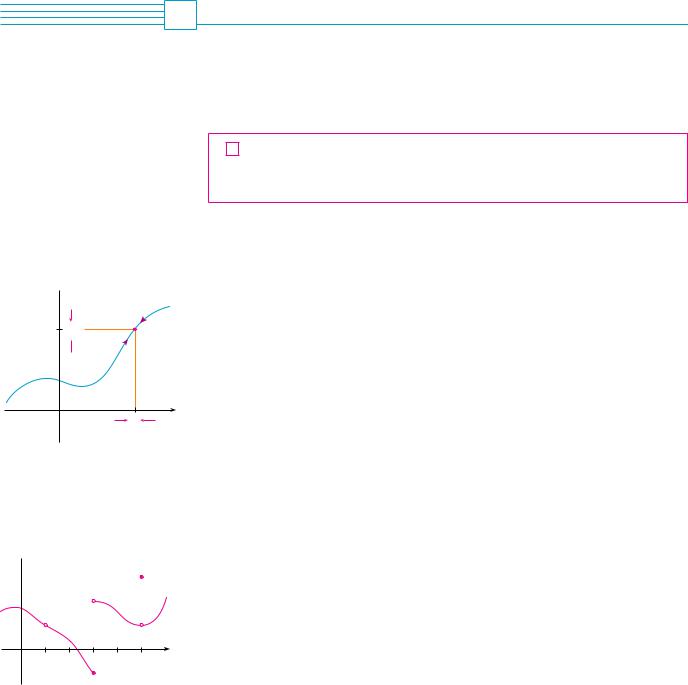
N As illustrated in Figure 1, if f is continuous, then the points "x, f "x## on the graph of f approach the point "a, f "a## on the graph. So there is no gap in the curve.
y y=Ä
y=Ä
Ä
approaches f(a) f(a). 
0 |
a |
x |
As x approaches a,
FIGURE 1
y
0 |
1 |
2 |
3 |
4 |
5 |
x |
FIGURE 2
We noticed in Section 2.3 that the limit of a function as x approaches a can often be found simply by calculating the value of the function at a. Functions with this property are called continuous at a. We will see that the mathematical definition of continuity corresponds closely with the meaning of the word continuity in everyday language. (A continuous process is one that takes place gradually, without interruption or abrupt change.)
1 DEFINITION A function f is continuous at a number a if
lim f "x# ! f "a#
x la
Notice that Definition l implicitly requires three things if f is continuous at a:
1.f "a# is defined (that is, a is in the domain of f )
2.lim f "x# exists
xla
3.lim f "x# ! f "a#
xla
The definition says that f is continuous at a if f "x# approaches f "a# as x approaches a. Thus a continuous function f has the property that a small change in x produces only a small change in f "x#. In fact, the change in f "x# can be kept as small as we please by keeping the change in x sufficiently small.
If f is defined near a (in other words, f is defined on an open interval containing a, except perhaps at a), we say that f is discontinuous at a (or f has a discontinuity at a) if f is not continuous at a.
Physical phenomena are usually continuous. For instance, the displacement or velocity of a vehicle varies continuously with time, as does a person’s height. But discontinuities do occur in such situations as electric currents. [See Example 6 in Section 2.2, where the Heaviside function is discontinuous at 0 because limt l0 H"t# does not exist.]
Geometrically, you can think of a function that is continuous at every number in an interval as a function whose graph has no break in it. The graph can be drawn without removing your pen from the paper.
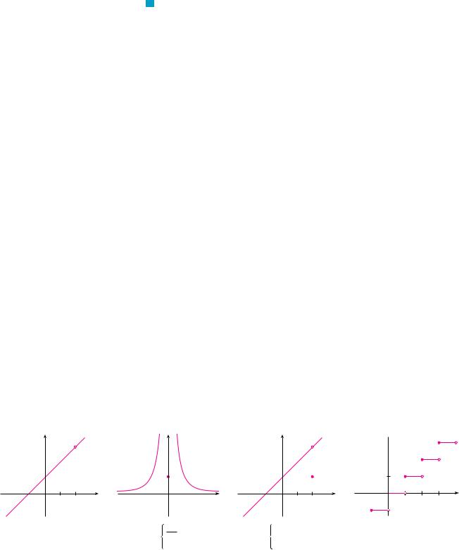
EXAMPLE 1 Figure 2 shows the graph of a function f. At which numbers is f discontinuous? Why?
SOLUTION It looks as if there is a discontinuity when a ! 1 because the graph has a break there. The official reason that f is discontinuous at 1 is that f "1# is not defined.
The graph also has a break when a ! 3, but the reason for the discontinuity is different. Here, f "3# is defined, but limx l3 f "x# does not exist (because the left and right limits are different). So f is discontinuous at 3.
What about a ! 5? Here, f "5# is defined and limx l5 f "x# exists (because the left and right limits are the same). But
|
lim f "x# " f "5# |
|
x l5 |
So f is discontinuous at 5. |
M |
Now let’s see how to detect discontinuities when a function is defined by a formula.
120 |||| CHAPTER 2 LIMITS AND DERIVATIVES
V EXAMPLE 2 Where are each of the following functions discontinuous?
|
x2 |
! x ! 2 |
|
|
|
1 |
if x " 0 |
|
(a) f "x# ! |
|
(b) f "x# ! -1x2 |
||||||
|
|
x ! 2 |
|
if x ! 0 |
||||
|
|
x |
2 ! x ! 2 |
if x " 2 |
|
|
|
|
(c) f "x# ! - |
|
x ! 2 |
(d) f "x# ! 0 x1 |
|
||||
1 |
if x ! 2 |
|
||||||
SOLUTION
(a)Notice that f "2# is not defined, so f is discontinuous at 2. Later we’ll see why f is continuous at all other numbers.
(b)Here f "0# ! 1 is defined but
lim f "x# ! lim |
1 |
||
x2 |
|||
x l0 |
x l0 |
||
does not exist. (See Example 8 in Section 2.2.) So f is discontinuous at 0.
(c) Here f "2# ! 1 is defined and |
|
|
|
|||
lim |
f "x# ! lim |
x2 |
! x ! 2 |
! lim |
"x ! 2#"x & 1# |
! lim "x & 1# ! 3 |
|
x ! 2 |
x ! 2 |
||||
x l2 |
x l2 |
|
x l2 |
x l2 |
||
exists. But
lim f "x# " f "2#
x l2
so f is not continuous at 2.
(d) The greatest integer function f "x# ! 0x1 has discontinuities at all of the integers because limx ln 0x1 does not exist if n is an integer. (See Example 10 and Exercise 49 in Section 2.3.) M
Figure 3 shows the graphs of the functions in Example 2. In each case the graph can’t be drawn without lifting the pen from the paper because a hole or break or jump occurs in the graph. The kind of discontinuity illustrated in parts (a) and (c) is called removable because we could remove the discontinuity by redefining f at just the single number 2. [The function t"x# ! x & 1 is continuous.] The discontinuity in part (b) is called an infinite discontinuity. The discontinuities in part (d) are called jump discontinuities because the function “jumps” from one value to another.
y |
|
|
y |
|
y |
|
|
|
1 |
|
|
1 |
|
1 |
|
|
|
0 |
1 2 |
x |
0 |
x |
0 |
1 |
2 |
x |
(a) Ä= |
≈-x-2 |
|
1 |
if x≠0 |
≈-x-2 |
if x≠2 |
||
x-2 |
|
(b) Ä= ≈ |
|
(c) Ä= |
x-2 |
|
|
|
|
|
1 |
if x=0 |
1 |
|
if x=2 |
||
|
|
|
|
|||||
FIGURE 3 Graphs of the functions in Example 2
y
1
0 1 2 3 x
(d) Ä=[x]
y
Д=1-Пггггг1-≈
1
|
|
|
|
|
|
|
|
- |
|
1 0 |
1 |
x |
|||
FIGURE 4
SECTION 2.5 CONTINUITY |||| 121
2 DEFINITION A function f is continuous from the right at a number a if
lim f "x# ! f "a#
x la&
and f is continuous from the left at a if
lim f "x# ! f "a#
x la!
EXAMPLE 3 At each integer n, the function f "x# ! 0 x1 [see Figure 3(d)] is continuous from the right but discontinuous from the left because
lim f "x# ! lim 0x1 ! n ! f "n#
|
|
x ln& |
|
|
|
x ln& |
|
|
|
|||||||
but |
|
lim f "x# ! lim 0 x1 ! n ! 1 " f "n# |
M |
|||||||||||||
|
|
x ln! |
|
|
x ln! |
|
|
|
||||||||
|
|
|
|
|||||||||||||
3 |
DEFINITION A function f |
is continuous on an interval if it is continuous at |
|
|||||||||||||
every number in the interval. (If f is defined only on one side of an endpoint of the |
|
|||||||||||||||
interval, we understand continuous at the endpoint to mean continuous from the |
|
|||||||||||||||
right or continuous from the left.) |
|
|
|
|
|
|
|
|
|
|
|
|||||
|
|
|
|
|||||||||||||
EXAMPLE 4 Show that the function f "x# ! 1 ! s |
|
|
|
is continuous on the |
|
|||||||||||
1 ! x2 |
|
|||||||||||||||
interval *!1, 1+. |
|
|
|
|
|
|
|
|
|
|
|
|
|
|
|
|
SOLUTION |
If !1 " a " 1, then using the Limit Laws, we have |
|
||||||||||||||
|
lim f "x# ! lim (1 ! |
s |
|
) |
|
|
|
|||||||||
|
1 ! x2 |
|
|
|
||||||||||||
|
x la |
x la |
|
|
|
|
|
|
|
|
|
|||||
|
|
! 1 ! lim |
|
|
|
|
|
|
|
|||||||
|
|
|
1 ! x2 |
|
|
|
(by Laws 2 and 7) |
|
||||||||
|
|
|
x la s |
|
|
|
|
|
|
|
|
|
|
|||
|
|
! 1 ! s |
|
|
|
|
|
|
|
|
||||||
|
|
xlimla "1 ! x2 # |
(by 11) |
|
||||||||||||
|
|
! 1 ! s |
|
|
|
|
|
|
|
|
|
|||||
|
|
1 ! a2 |
(by 2, 7, and 9) |
|
||||||||||||
|
|
! f "a# |
|
|
|
|
|
|
|
|
|
|
|
|||
Thus, by Definition l, f is continuous at a if !1 " a " 1. Similar calculations show that
lim f "x# ! 1 ! f "!1# and |
lim f "x# ! 1 ! f "1# |
x l!1& |
xl1! |
so f is continuous from the right at !1 and continuous from the left at 1. Therefore, according to Definition 3, f is continuous on *!1, 1+.
The graph of f is sketched in Figure 4. It is the lower half of the circle |
|
x2 & " y ! 1#2 ! 1 |
M |
Instead of always using Definitions 1, 2, and 3 to verify the continuity of a function as we did in Example 4, it is often convenient to use the next theorem, which shows how to build up complicated continuous functions from simple ones.
122 |||| CHAPTER 2 LIMITS AND DERIVATIVES
4 |
THEOREM |
If f and t are continuous at a and c is a constant, then the follow- |
|||
ing functions are also continuous at a: |
|
||||
1. |
f ! t |
2. |
f " t |
3. cf |
|
4. |
ft |
5. |
f |
if t!a" " 0 |
|
t |
|
||||
|
|
|
|
|
|
P R O O F Each of the five parts of this theorem follows from the corresponding Limit Law in Section 2.3. For instance, we give the proof of part 1. Since f and t are continuous at a, we have
|
lim f !x" ! f !a" |
and |
lim t!x" ! t!a" |
|
|
x la |
|
x la |
|
Therefore |
|
|
|
|
lim ! f ! t"!x" ! lim $ f !x" ! t!x"% |
|
|||
x la |
x la |
|
|
|
|
! lim f !x" ! lim t!x" |
(by Law 1) |
||
|
x la |
|
x la |
|
! f !a" ! t!a" ! ! f ! t"!a"
This shows that f ! t is continuous at a.
M
It follows from Theorem 4 and Definition 3 that if f and t are continuous on an interval, then so are the functions f ! t, f " t, cf, ft, and (if t is never 0) f#t. The following theorem was stated in Section 2.3 as the Direct Substitution Property.
5 THEOREM
(a)Any polynomial is continuous everywhere; that is, it is continuous on
! ! !"$, $".
(b)Any rational function is continuous wherever it is defined; that is, it is continuous on its domain.
P R O O F
(a) A polynomial is a function of the form
P!x" ! cn xn ! cn"1xn"1 ! ### ! c1x ! c0
where c0, c1, . . . , cn are constants. We know that
|
lim c0 ! c0 |
(by Law 7) |
|
|
|
x la |
|
|
|
and |
lim xm ! am |
m ! 1, 2, . . . , n |
(by 9) |
|
|
x la |
|
|
|
This equation is precisely the statement that the function f !x" ! xm is a continuous function. Thus, by part 3 of Theorem 4, the function t!x" ! cxm is continuous. Since P is a sum of functions of this form and a constant function, it follows from part 1 of Theorem 4 that P is continuous.
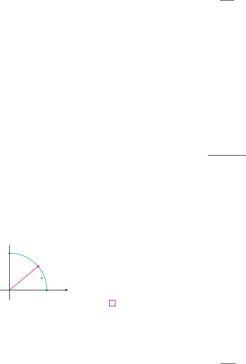
y
P(cos!¬,!sin!¬) 1 
¬
0(1,!0) x
FIGURE 5
N Another way to establish the limits in (6) is to use the Squeeze Theorem with the inequality sin % ( % (for % ' 0), which is proved in Section 3.3.
SECTION 2.5 CONTINUITY |||| 123
(b) A rational function is a function of the form
f !x" ! P!x" Q!x"
where P and Q are polynomials. The domain of f is D ! 'x ! ! & Q!x" " 0(. We know from part (a) that P and Q are continuous everywhere. Thus, by part 5 of Theorem 4,
f is continuous at every number in D. M
As an illustration of Theorem 5, observe that the volume of a sphere varies continuously with its radius because the formula V!r" ! 43 &r3 shows that V is a polynomial function of r. Likewise, if a ball is thrown vertically into the air with a velocity of 50 ft#s, then the height of the ball in feet t seconds later is given by the formula h ! 50t " 16t2. Again this is a polynomial function, so the height is a continuous function of the elapsed time.
Knowledge of which functions are continuous enables us to evaluate some limits very quickly, as the following example shows. Compare it with Example 2(b) in Section 2.3.
EXAMPLE 5 Find |
lim |
x3 |
! 2x2 " 1 |
. |
|
|
5 |
" 3x |
|||
|
x l"2 |
|
|
||
SOLUTION The function
f !x" ! x3 ! 2x2 " 1 5 " 3x
is rational, so by Theorem 5 it is continuous on its domain, which is {x & x " 53}. Therefore
lim |
x3 |
! 2x2 " 1 |
! lim f !x" ! f !"2" |
|
|
|
||
|
5 |
" 3x |
|
|
|
|||
x l"2 |
|
|
x l"2 |
|
|
|
||
|
|
|
|
! |
!"2"3 ! 2!"2"2 " 1 |
! " |
1 |
M |
|
|
|
|
5 " 3!"2" |
11 |
|||
It turns out that most of the familiar functions are continuous at every number in their domains. For instance, Limit Law 10 (page 101) is exactly the statement that root functions are continuous.
From the appearance of the graphs of the sine and cosine functions (Figure 18 in Section 1.2), we would certainly guess that they are continuous. We know from the definitions of sin % and cos % that the coordinates of the point P in Figure 5 are !cos %, sin %". As
% l 0, we see that P approaches the point !1, 0" and so cos % l 1 and sin % l 0. Thus |
||
6 |
lim cos % ! 1 |
lim sin % ! 0 |
|
%l0 |
%l0 |
Since cos 0 ! 1 and sin 0 ! 0, the equations in (6) assert that the cosine and sine functions are continuous at 0. The addition formulas for cosine and sine can then be used to deduce that these functions are continuous everywhere (see Exercises 56 and 57).
It follows from part 5 of Theorem 4 that
tan x ! sin x cos x

124 |||| CHAPTER 2 LIMITS AND DERIVATIVES
|
|
|
|
|
|
|
|
|
|
y |
|
|
|
|
|
|
|
|
|
|
|
is continuous except where cos x ! 0. This happens when x is an odd integer multiple of |
|||||||||||||
|
|
|
|
|
|
|
|
|
|
|
|
|
|
|
|
|
|
|
|
|
|
|
, so y ! tan x has infinite discontinuities when x ! *, *3, *5, and so on |
||||||||||||
|
|
|
|
|
|
|
|
|
|
|
|
|
|
|
|
|
|
|
|
|
|
|
(see Figure 6). |
|
|
|
|
|
|
|
|
|
|
||
|
|
|
|
|
|
|
|
1 |
|
|
|
|
|
|
|
|
|
|
|
|
The inverse function of any continuous one-to-one function is also continuous. (This |
||||||||||||||
|
|
|
|
|
|
|
|
|
|
|
|
|
|
|
|
|
|
|
|
fact is proved in Appendix F, but our geometric intuition makes it seem plausible: The |
|||||||||||||||
|
|
|
|
|
|
|
|
|
|
|
|
|
|
|
|
|
|
|
|
|
|
|
|||||||||||||
_ |
3 |
|
π |
_π |
_ |
π |
0 |
π |
π |
3π |
x |
graph of f "1 is obtained by reflecting the graph of f about the line y ! x. So if the graph |
|||||||||||||||||||||||
2 |
2 |
|
|
2 |
2 |
|
of f has no break in it, neither does the graph of f |
"1 |
.) Thus the inverse trigonometric func- |
||||||||||||||||||||||||||
|
|
|
|
|
|
|
|
|
|
|
|
||||||||||||||||||||||||
|
|
|
|
|
|
|
|
|
|
|
|
|
|
|
|
|
|
|
|
|
|
|
tions are continuous. |
|
|
|
|
|
|
|
|
|
|
||
|
|
|
|
|
|
|
|
|
|
|
|
|
|
|
|
|
|
|
|
|
|
|
In Section 1.5 we defined the exponential function y ! ax so as to fill in the holes in the |
||||||||||||
|
|
|
|
|
|
|
|
|
|
|
|
|
|
|
|
|
|
|
|
|
|
|
graph of y ! ax where x is rational. In other words, the very definition of y ! ax makes |
||||||||||||
FIGURE 6 |
y=tan x |
|
|
|
|
|
|
|
|
|
|
it a continuous function on !. Therefore its inverse function y ! loga x is continuous |
|||||||||||||||||||||||
|
|
|
|
|
|
|
|
|
|
on !0, $". |
|
|
|
|
|
|
|
|
|
|
|||||||||||||||
|
|
|
|
|
|
|
|
|
|
|
|
|
|
|
|
|
|
||||||||||||||||||
N The inverse trigonometric functions are |
7 |
THEOREM The following types of functions are continuous at every number in |
|
||||||||||||||||||||||||||||||||
reviewed in Section 1.6. |
|
|
|
|
|
|
|
|
|
|
|
their domains: |
|
|
|
|
|
|
|
|
|
|
|||||||||||||
|
|
|
|
|
|
|
|
|
|
|
|
|
|
|
|
|
|
|
|
|
|
|
|
polynomials |
rational functions |
|
|
root functions |
|
||||||
|
|
|
|
|
|
|
|
|
|
|
|
|
|
|
|
|
|
|
|
|
|
|
|
trigonometric functions |
inverse trigonometric functions |
|
|||||||||
|
|
|
|
|
|
|
|
|
|
|
|
|
|
|
|
|
|
|
|
|
|
|
|
exponential functions |
|
|
|
logarithmic functions |
|
||||||
|
|
|
|
|
|
|
|
|
|
|
|
|
|
|
|
|
|
|
|
|
|
|
|
|
|
|
|||||||||
|
|
|
|
|
|
|
|
|
|
|
|
|
|
|
|
|
|
|
|
|
|
|
EXAMPLE 6 Where is the function f !x" ! |
ln x ! tan"1x |
continuous? |
|
|||||||||
|
|
|
|
|
|
|
|
|
|
|
|
|
|
|
|
|
|
|
|
|
|
|
|
|
|||||||||||
|
|
|
|
|
|
|
|
|
|
|
|
|
|
|
|
|
|
|
|
|
|
|
|
|
|
|
|
|
|
x2 " 1 |
|
|
|||
|
|
|
|
|
|
|
|
|
|
|
|
|
|
|
|
|
|
|
|
|
|
|
SOLUTION |
We know from Theorem 7 that the function y ! ln x is continuous for x ' 0 |
|
||||||||||
|
|
|
|
|
|
|
|
|
|
|
|
|
|
|
|
|
|
|
|
|
|
|
and y ! tan"1x is continuous on !. Thus, by part 1 of Theorem 4, y ! ln x ! tan"1x is |
|
|||||||||||
|
|
|
|
|
|
|
|
|
|
|
|
|
|
|
|
|
|
|
|
|
|
|
continuous on !0, $". The denominator, y ! x2 " 1, is a polynomial, so it is continuous |
||||||||||||
|
|
|
|
|
|
|
|
|
|
|
|
|
|
|
|
|
|
|
|
|
|
|
everywhere. Therefore, by part 5 of Theorem 4, f is continuous at all positive numbers x |
||||||||||||
|
|
|
|
|
|
|
|
|
|
|
|
|
|
|
|
|
|
|
|
|
|
|
except where x2 " 1 ! 0. So f is continuous on the intervals !0, 1" and !1, $". |
M |
|||||||||||
|
|
|
|
|
|
|
|
|
|
|
|
|
|
|
|
|
|
|
|
|
|
|
EXAMPLE 7 Evaluate lim |
|
sin x |
|
. |
|
|
|
|
|
|
|
|
|
|
|
|
|
|
|
|
|
|
|
|
|
|
|
|
|
|
|
|
|
|
|
|
! cos x |
|
|
|
|
|
|
|
||||
|
|
|
|
|
|
|
|
|
|
|
|
|
|
|
|
|
|
|
|
|
|
|
|
x l& 2 |
|
|
|
|
|
|
|
|
|||
|
|
|
|
|
|
|
|
|
|
|
|
|
|
|
|
|
|
|
|
|
|
|
SOLUTION |
Theorem 7 tells us that y ! sin x is continuous. The function in the denomi- |
|
||||||||||
|
|
|
|
|
|
|
|
|
|
|
|
|
|
|
|
|
|
|
|
|
|
|
nator, y ! 2 ! cos x, is the sum of two continuous functions and is therefore continu- |
|
|||||||||||
|
|
|
|
|
|
|
|
|
|
|
|
|
|
|
|
|
|
|
|
|
|
|
ous. Notice that this function is never 0 because cos x ) "1 for all x and so |
|
|||||||||||
|
|
|
|
|
|
|
|
|
|
|
|
|
|
|
|
|
|
|
|
|
|
|
2 ! cos x ' 0 everywhere. Thus the ratio |
|
|
|
|
|
|
||||||
|
|
|
|
|
|
|
|
|
|
|
|
|
|
|
|
|
|
|
|
|
|
|
|
|
|
|
f !x" ! |
sin x |
|
|
|
|
|||
|
|
|
|
|
|
|
|
|
|
|
|
|
|
|
|
|
|
|
|
|
|
|
|
|
|
|
2 ! cos x |
|
|
||||||
|
|
|
|
|
|
|
|
|
|
|
|
|
|
|
|
|
|
|
|
|
|
|
|
|
|
|
|
|
|
|
|
||||
is continuous everywhere. Hence, by definition of a continuous function,
lim
x l&
2
sin x
! cos x !
lim f !x" ! f !&" !
x l&
sin &
2 ! cos
&
! 2 "0 1 ! 0
M
Another way of combining continuous functions f and t to get a new continuous function is to form the composite function f " t. This fact is a consequence of the following theorem.
N This theorem says that a limit symbol can be moved through a function symbol if the function is continuous and the limit exists. In other words, the order of these two symbols can be reversed.
SECTION 2.5 CONTINUITY |||| 125
8 THEOREM If f is continuous at b and lim t!x" ! b, |
then lim f ! t!x"" ! f !b". |
|||
In other words, |
x la |
|
x la |
|
|
|
) |
|
|
|
lim f ! t!x"" ! f |
lim t!x" |
|
|
|
x la |
(x la |
|
|
Intuitively, Theorem 8 is reasonable because if x is close to a, then t!x" and since f is continuous at b, if t!x" is close to b, then f ! t!x"" is close to of Theorem 8 is given in Appendix F.
|
|
1 " s |
|
|
|
|
|
EXAMPLE 8 Evaluate lim arcsin |
|
x |
. |
||||
) |
1 " x * |
||||||
x l1 |
|
||||||
SOLUTION Because arcsin is a continuous function, we can apply Theorem 8:
|
|
1 " s |
|
|
|
|
|
|
|
1 " s |
|
|
|
||||||||||||
lim arcsin |
|
x |
|
|
! arcsin |
|
lim |
x |
|||||||||||||||||
) |
1 " x |
* |
|
1 " x * |
|||||||||||||||||||||
x l1 |
|
)x l1 |
|
||||||||||||||||||||||
|
|
|
|
|
|
|
|
|
|
|
|
|
1 " s |
|
|
|
|
|
|||||||
|
|
|
|
|
|
! arcsin |
|
lim |
|
|
|
x |
|||||||||||||
|
|
|
|
|
|
|
|
|
|
|
|
|
|
|
|
|
|
|
|
|
|
|
|||
|
|
|
|
|
|
|
)x l1 |
(1 " sx ) (1 ! sx )* |
|||||||||||||||||
|
|
|
|
|
|
! arcsin |
|
lim |
|
1 |
|
|
|
|
|
|
|
|
|
|
|
|
|||
|
|
|
|
|
|
|
|
|
|
|
|
|
|
|
|
|
|
|
|
|
|
|
|||
|
|
|
|
|
|
|
|
|
|
|
|
|
|
|
|
|
|
|
|
|
|
|
|||
|
|
|
|
|
|
|
)x l1 |
1 ! sx * |
|||||||||||||||||
|
|
|
|
|
|
! arcsin |
1 |
! |
|
& |
|
|
|
|
|
|
|
|
|
|
|
|
|
||
|
|
|
|
|
|
|
2 |
|
6 |
|
|
|
|
|
|
|
|
|
|
|
|
|
|||
is close to b, f !b". A proof
M
Let’s now apply Theorem 8 in the special case where f !x" ! sn x , with n being a positive integer. Then
|
f ! t!x"" ! s |
|
|
|||||||
|
t!x" |
|||||||||
|
|
|
|
|
n |
|
|
|
|
|
and |
f (xlimla t!x") ! sn |
|
|
|
||||||
xlimla t!x" |
||||||||||
If we put these expressions into Theorem 8, we get |
||||||||||
|
lim s |
|
|
|
|
|
|
|
|
|
|
t!x" |
! |
n |
|
lim t!x" |
|||||
|
n |
|
|
|
|
|
|
|||
|
x la |
sx la |
||||||||
and so Limit Law 11 has now been proved. (We assume that the roots exist.)
9 THEOREM If t is continuous at a and f is continuous at t!a", then the composite function f " t given by ! f " t"!x" ! f ! t!x"" is continuous at a.
This theorem is often expressed informally by saying “a continuous function of a continuous function is a continuous function.”
P R O O F Since t is continuous at a, we have
lim t!x" ! t!a"
x la
Since f is continuous at b ! t!a", we can apply Theorem 8 to obtain lim f ! t!x"" ! f ! t!a""
x la
126 |||| CHAPTER 2 LIMITS AND DERIVATIVES
which is precisely the statement that the function h!x" ! f ! t!x"" is continuous at a; that
is, f " t is continuous at a. |
M |
||
|
EXAMPLE 9 Where are the following functions continuous? |
||
V |
|||
(a) |
h!x" ! sin!x2 " |
(b) F!x" ! ln!1 ! cos x" |
|
SOLUTION |
|
||
(a) |
We have h!x" ! f ! t!x"", where |
|
|
2 |
_10 |
_6 |
FIGURE 7 y=ln(1+cos x)
t!x" ! x2 and f !x" ! sin x
10Now t is continuous on ! since it is a polynomial, and f is also continuous everywhere. Thus h ! f " t is continuous on ! by Theorem 9.
(b) We know from Theorem 7 that f !x" ! ln x is continuous and t!x" ! 1 ! cos x is continuous (because both y ! 1 and y ! cos x are continuous). Therefore, by Theorem 9, F!x" ! f ! t!x"" is continuous wherever it is defined. Now ln!1 ! cos x" is defined when 1 ! cos x ' 0. So it is undefined when cos x ! "1, and this happens
when x ! *&, *3&, . . . . Thus F has discontinuities when x is an odd multiple of & and is continuous on the intervals between these values (see Figure 7). M
An important property of continuous functions is expressed by the following theorem, whose proof is found in more advanced books on calculus.
10 THE INTERMEDIATE VALUE THEOREM Suppose that f is continuous on the closed interval $a, b% and let N be any number between f !a" and f !b", where f !a" " f !b". Then there exists a number c in !a, b" such that f !c" ! N.
The Intermediate Value Theorem states that a continuous function takes on every intermediate value between the function values f !a" and f !b". It is illustrated by Figure 8. Note that the value N can be taken on once [as in part (a)] or more than once [as in part (b)].
y |
|
|
|
y |
|
|
|
|
|
f(b) |
|
|
|
f(b) |
|
|
y=Ä |
|
|
N |
|
|
|
|
|
|
|
|
|
|
|
|
N |
|
|
|
|
|
|
|
|
|
|
|
|
|
|
|
|
f(a) |
|
y=Ä |
|
f(a) |
|
|
|
|
|
0 |
a |
c b |
x |
0 |
a cÁ |
cª |
c£ |
b |
x |
FIGURE 8 |
(a) |
|
|
|
|
(b) |
|
|
|
y
|
f(a) |
|
|
|
y=Ä |
If we think of a continuous function as a function whose graph has no hole or break, |
|||
|
|
|
|
||||||
|
|
|
|
|
then it is easy to believe that the Intermediate Value Theorem is true. In geometric terms it |
||||
|
N |
|
|
|
y=N |
||||
|
|
|
|
says that if any horizontal line y ! N is given between y ! f !a" and y ! f !b" as in Fig- |
|||||
|
|
|
|
|
|
|
|
|
|
|
f(b) |
|
|
|
|
|
|
|
ure 9, then the graph of f can’t jump over the line. It must intersect y ! N somewhere. |
|
|
|
|
|
|
|
|
It is important that the function f in Theorem 10 be continuous. The Intermediate Value |
|
|
|
|
|
|
|
|
|
||
0 |
|
a |
b x |
Theorem is not true in general for discontinuous functions (see Exercise 44). |
|||||
|
|
|
|
|
|
|
|
|
One use of the Intermediate Value Theorem is in locating roots of equations as in the |
FIGURE 9 |
|
|
|
|
following example. |
||||
SECTION 2.5 CONTINUITY |||| 127
V EXAMPLE 10 Show that there is a root of the equation
4x3 " 6x2 ! 3x " 2 ! 0
between 1 and 2.
SOLUTION Let f !x" ! 4x3 " 6x2 ! 3x " 2. We are looking for a solution of the given equation, that is, a number c between 1 and 2 such that f !c" ! 0. Therefore, we take a ! 1, b ! 2, and N ! 0 in Theorem 10. We have
|
f !1" ! 4 " 6 ! 3 " 2 ! "1 ( 0 |
and |
f !2" ! 32 " 24 ! 6 " 2 ! 12 ' 0 |
Thus f !1" ( 0 ( f !2"; that is, N ! 0 is a number between f !1" and f !2". Now f is continuous since it is a polynomial, so the Intermediate Value Theorem says there is a number c between 1 and 2 such that f !c" ! 0. In other words, the equation
4x3 " 6x2 ! 3x " 2 ! 0 has at least one root c in the interval !1, 2".
In fact, we can locate a root more precisely by using the Intermediate Value Theorem again. Since
f !1.2" ! "0.128 ( 0 and f !1.3" ! 0.548 ' 0
a root must lie between 1.2 and 1.3. A calculator gives, by trial and error,
f !1.22" ! "0.007008 ( 0 and f !1.23" ! 0.056068 ' 0
so a root lies in the interval !1.22, 1.23".
M
We can use a graphing calculator or computer to illustrate the use of the Intermediate Value Theorem in Example 10. Figure 10 shows the graph of f in the viewing rectangle $"1, 3% by $"3, 3% and you can see that the graph crosses the x-axis between 1 and 2. Figure 11 shows the result of zooming in to the viewing rectangle $1.2, 1.3% by $"0.2, 0.2%.
3 |
|
0.2 |
|
|||
_1 |
|
|
3 |
1.2 |
|
1.3 |
|
|
|
||||
|
|
|
_0.2 |
|
||
_3 |
|
|
||||
FIGURE 10 |
|
FIGURE 11 |
|
|||
In fact, the Intermediate Value Theorem plays a role in the very way these graphing devices work. A computer calculates a finite number of points on the graph and turns on the pixels that contain these calculated points. It assumes that the function is continuous and takes on all the intermediate values between two consecutive points. The computer therefore connects the pixels by turning on the intermediate pixels.
128|||| CHAPTER 2 LIMITS AND DERIVATIVES
2.5EXERCISES
1.Write an equation that expresses the fact that a function f is continuous at the number 4.
2.If f is continuous on !"$, $", what can you say about its graph?
3.(a) From the graph of f, state the numbers at which f is discontinuous and explain why.
(b)For each of the numbers stated in part (a), determine whether f is continuous from the right, or from the left, or neither.
y
_4 |
_2 |
0 |
2 |
4 |
6 |
x |
||||||||||
4.From the graph of t, state the intervals on which t is continuous.
y
_4 |
_2 |
2 |
4 |
6 |
8 x |
||||||||||||
5.Sketch the graph of a function that is continuous everywhere except at x ! 3 and is continuous from the left at 3.
6.Sketch the graph of a function that has a jump discontinuity at x ! 2 and a removable discontinuity at x ! 4, but is continuous elsewhere.
7.A parking lot charges $3 for the first hour (or part of an hour) and $2 for each succeeding hour (or part), up to a daily maximum of $10.
(a)Sketch a graph of the cost of parking at this lot as a function of the time parked there.
(b)Discuss the discontinuities of this function and their significance to someone who parks in the lot.
8.Explain why each function is continuous or discontinuous.
(a)The temperature at a specific location as a function of time
(b)The temperature at a specific time as a function of the distance due west from New York City
(c)The altitude above sea level as a function of the distance due west from New York City
(d)The cost of a taxi ride as a function of the distance traveled
(e)The current in the circuit for the lights in a room as a function of time
9.If f and t are continuous functions with f !3" ! 5 and limx l3 $2 f !x" " t!x"% ! 4, find t!3".
10–12 Use the definition of continuity and the properties of limits to show that the function is continuous at the given number a.
10.f !x" ! x2 ! s7 " x , a ! 4
11.f !x" ! !x ! 2x3 "4, a ! "1
2t " 3t2
12. h!t" ! 1 ! t3 , a ! 1
13–14 Use the definition of continuity and the properties of limits to show that the function is continuous on the given interval.
13. |
f !x" ! |
2x ! 3 |
, |
|
!2, $" |
|
x " 2 |
|
|||||
|
|
|
|
|
||
14. |
t!x" ! 2 s |
|
, |
!"$, 3% |
||
3 " x |
||||||
|
|
|
|
|
|
|
15–20 Explain why the function is discontinuous at the given number a. Sketch the graph of the function.
15. |
f !x" ! ln & x " 2 & |
a ! 2 |
||||||
|
|
|
|
1 |
|
if x " 1 |
|
|
16. |
f !x" ! +2x " 1 |
a ! 1 |
||||||
if x ! 1 |
||||||||
|
|
|
ex |
if |
x ( 0 |
|
||
17. |
f !x" ! +x2 |
if |
x ) 0 |
a ! 0 |
||||
|
|
|
x2 " x |
if x " 1 |
|
|||
18. |
f !x" ! +1x2 " 1 |
a ! 1 |
||||||
if x ! 1 |
||||||||
|
|
|
cos x |
if x ( 0 |
|
|||
19. |
f !x" ! |
0 |
|
|
if x ! 0 |
a ! 0 |
||
|
|
+1 " x2 |
if x ' 0 |
|
||||
|
2x2 " 5x " 3 |
if x " 3 |
|
||
20. f !x" ! +6 |
x " 3 |
a ! 3 |
|||
if x ! 3 |
|||||
21–28 Explain, using Theorems 4, 5, 7, and 9, why the function is continuous at every number in its domain. State the domain.
|
|
|
x |
|
3 |
|
|
3 |
|
|
|
|
|
|
|
|
|||
21. F!x" ! |
x |
2 |
! 5x ! 6 |
22. |
G!x" ! sx !1 |
! x |
" |
||
|
|
|
|
|
|
|
|
||
23. |
R!x" ! x2 ! s |
|
|
24. |
h!x" ! |
sin x |
|
|
2x " 1 |
|
|||||||
x ! 1 |
||||||||
|
|
|
|
|
|
|||
25. |
L!t" ! e"5t cos 2&t |
26. |
F!x" ! sin"1!x2 " 1" |
|||||
27. |
G!t" ! ln!t4 " 1" |
28. |
H!x" ! cos(esx ) |
|||||
;29–30 Locate the discontinuities of the function and illustrate by graphing.
29. y ! |
|
1 |
30. |
y ! ln!tan2x" |
|
1 |
! e1#x |
||||
|
|
|
31–34 Use continuity to evaluate the limit.
31. |
lim |
5 ! s |
x |
|
32. |
lim sin!x ! sin x" |
|
||||
|
|
|
|
|
|||||||
|
x l4 |
s5 ! x |
|
|
x l |
|
|
|
|||
|
|
|
|
|
|
|
& |
|
|
|
|
|
|
2 |
|
|
|
|
|
|
x2 " 4 |
|
|
33. |
lim ex |
"x |
34. |
lim arctan |
|
|
|
||||
)3x2 " 6x |
* |
||||||||||
|
x l1 |
|
|
|
|
|
x l2 |
||||
35–36 Show that
35. f !x" ! +sxx2
+sin x
36. f !x" ! cos x
f is continuous on !"$, $".
if x ( 1 if x ) 1
if x ( 4 if x ) 4
37–39 Find the numbers at which f is discontinuous. At which
of these numbers is f |
continuous from the right, from the left, or |
||||||
neither? Sketch the graph of f. |
|||||||
|
|
1 |
|
! x2 |
if |
x + 0 |
|
37. |
f !x" ! |
2 |
|
" x |
if |
0 ( x + 2 |
|
|
|
+!x " 2"2 if x ' 2 |
|||||
|
|
x ! 1 |
if |
x + 1 |
|||
38. |
f !x" ! |
1#x |
if 1 ( x ( 3 |
||||
|
|
+s |
|
|
if |
x ) 3 |
|
|
|
x " 3 |
|||||
|
|
x ! 2 |
if x ( 0 |
||||
39. |
f !x" ! |
ex |
|
|
if 0 + x + 1 |
||
|
|
+2 |
|
" x |
if x ' 1 |
||
40.The gravitational force exerted by the earth on a unit mass at a distance r from the center of the planet is
|
GMr |
if r ( R |
|
R3 |
|
F!r" ! |
|
|
GM |
if r ) R |
|
|
r2 |
|
|
|
where M is the mass of the earth, R is its radius, and G is the gravitational constant. Is F a continuous function of r?
SECTION 2.5 CONTINUITY |||| 129
41.For what value of the constant c is the function f continuous on !"$, $"?
cx2 ! 2x |
if x ( 2 |
f !x" ! +x3 " cx |
if x ) 2 |
42. Find the values of a and b that make f continuous everywhere.
x2 " 4
x " 2
if x ( 2
f !x" ! ax2 " bx ! 3 if 2 ( x ( 3
2x " a ! b if x ) 3
43.Which of the following functions f has a removable discontinuity at a? If the discontinuity is removable, find a function t that agrees with f for x " a and is continuous at a.
(a) f !x" ! |
x4 |
" 1 |
, |
a ! |
1 |
||
x |
" 1 |
||||||
|
|
|
|
|
|||
(b) f !x" ! |
x3 |
" x2 " 2x |
, |
a ! 2 |
|||
|
x " 2 |
|
|||||
|
|
|
|
|
|||
(c)f !x" ! , sin x- , a ! &
44.Suppose that a function f is continuous on [0, 1] except at 0.25 and that f !0" ! 1 and f !1" ! 3. Let N ! 2. Sketch two possible graphs of f , one showing that f might not satisfy the conclusion of the Intermediate Value Theorem and one showing that f might still satisfy the conclusion of the Intermediate Value Theorem (even though it doesn’t satisfy the hypothesis).
45.If f !x" ! x2 ! 10 sin x, show that there is a number c such that f !c" ! 1000.
46.Suppose f is continuous on $1, 5% and the only solutions of the equation f !x" ! 6 are x ! 1 and x ! 4. If f !2" ! 8, explain why f !3" ' 6.
47–50 Use the Intermediate Value Theorem to show that there is a root of the given equation in the specified interval.
47. |
x4 ! x " 3 ! 0, !1, 2" |
48. |
s |
|
! 1 " x, |
!0, 1" |
3 |
x |
|||||
49. |
cos x ! x, !0, 1" |
50. |
ln x ! e"x, |
!1, 2" |
||
|
|
|
|
|
|
|
51–52 (a) Prove that the equation has at least one real root.
(b) Use your calculator to find an interval of length 0.01 that contains a root.
51. cos x ! x3 52. ln x ! 3 " 2x
;53–54 (a) Prove that the equation has at least one real root.
(b) Use your graphing device to find the root correct to three decimal places.
|
|
100e"x#100 ! 0.01x2 |
54. arctan x ! 1 " x |
|
53. |
||
|
|
|
|