Добавил:

PavelEngineer Опубликованный материал нарушает ваши авторские права? Сообщите нам.

Вуз:

Севастопольский Государственный Университет

Предмет:

[НЕСОРТИРОВАННОЕ]

Файл:

[James_Stewart]_Single_Variable_Calculus_Early_Tr(BookFi).pdf

Скачиваний:

Добавлен:

30.12.2019

Размер:

18.09 Mб

Скачать

☆

<<< < Предыдущая 4 5 6 7 8 9 10 11 12 13 14 1516 / 9116 17 18 19 20 21 22 23 24 25 26 27 28 > Следующая >>>

;(b) Graph v"t# if v* ! 1 m!s and t ! 9.8 m!s2. How long does it take for the velocity of the raindrop to reach 99% of its terminal velocity?

;60. (a) By graphing y ! e"x!10 and y ! 0.1 on a common screen, discover how large you need to make x so that e"x!10 $ 0.1.

(b)Can you solve part (a) without using a graphing device?

;61. Use a graph to ﬁnd a number N such that

if	x % N then &	3x2 # 1	" 1.5 & $ 0.05
		2x2 # x # 1

;62. For the limit

lim s4x2 # 1 ! 2

x l! x # 1

illustrate Deﬁnition 7 by ﬁnding values of N that correspond to ( ! 0.5 and ( ! 0.1.

;63. For the limit

lim	s	4x2 # 1	! "2
		x # 1
x l"!

illustrate Deﬁnition 8 by ﬁnding values of N that correspond to ( ! 0.5 and ( ! 0.1.

;64. For the limit

lim	2x # 1	! !

x l! sx # 1

illustrate Deﬁnition 9 by ﬁnding a value of N that corresponds to M ! 100.

SECTION 2.7 DERIVATIVES AND RATES OF CHANGE |||| 143

65.(a) How large do we have to take x so that 1!x2 $ 0.0001?

(b) Taking r ! 2 in Theorem 5, we have the statement

lim x2 ! 0

x l!

Prove this directly using Deﬁnition 7.

66.(a) How large do we have to take x so that 1!sx $ 0.0001?

(b) Taking r ! 12 in Theorem 5, we have the statement

	lim	1		! 0
	lim			! 0
	x l!	sx
	Prove this directly using Deﬁnition 7.
67.	Use Deﬁnition 8 to prove that			lim	1	!	0.
67.	Use Deﬁnition 8 to prove that			lim		!	0.
			x l"!		x
68.	Prove, using Deﬁnition 9, that lim x3 ! !.
			x l!

69.Use Deﬁnition 9 to prove that lim ex ! !.

xl!

70.Formulate a precise deﬁnition of

lim f "x# ! "!

	x l"!
Then use your deﬁnition to prove that
	lim	"1 # x3 # ! "!
	x l"!
71. Prove that
	lim f "x# ! lim f "1!t#
	x l!	t l0#
and	lim	f "x# ! lim f "1!t#
	x l"!	t l0"

if these limits exist.

2.7 DERIVATIVES AND RATES OF CHANGE

The problem of ﬁnding the tangent line to a curve and the problem of ﬁnding the velocity of an object both involve ﬁnding the same type of limit, as we saw in Section 2.1. This special type of limit is called a derivative and we will see that it can be interpreted as a rate of change in any of the sciences or engineering.

TANGENTS

If a curve C has equation y ! f "x# and we want to ﬁnd the tangent line to C at the point P"a, f "a##, then we consider a nearby point Q"x, f "x##, where x " a, and compute the slope of the secant line PQ:

mPQ ! f "x# " f "a# x " a

Then we let Q approach P along the curve C by letting x approach a. If mPQ approaches a number m, then we deﬁne the tangent t to be the line through P with slope m. (This

144 |||| CHAPTER 2 LIMITS AND DERIVATIVES

y		Q{x,!Ä}		amounts to saying that the tangent line is the limiting position of the secant line PQ as Q
		Q{x,!Ä}	Ä-f(a)	approaches P. See Figure 1.)
	P{a,!f(a)}		Ä-f(a)
	P{a,!f(a)}			1	DEFINITION The tangent line to the curve y ! f "x# at the point P"a, f "a## is
				1
		x-a		the line through P with slope
					m ! lim f "x# " f "a#
0	a	x				x la	x " a
0	a	x	x	provided that this limit exists.
				provided that this limit exists.
y		t		In our ﬁrst example we conﬁrm the guess we made in Example 1 in Section 2.1.
		Q	Q	V EXAMPLE 1 Find an equation of the tangent line to the parabola y ! x2 at the
			Q	point P"1, 1#.
	P		Q	point P"1, 1#.
	P		Q	SOLUTION	Here we have a ! 1 and f "x# ! x2, so the slope is
					m ! lim	f "x# " f "1#		! lim	x2 " 1
					m ! lim	x " 1		! lim	x " 1
					x l1	x " 1		x l1	x " 1
0			x		! lim	"x " 1#"x # 1#
					x l1	x " 1

FIGURE 1

N Point-slope form for a line through the point "x1, y1# with slope m:

y " y1 ! m"x " x1#

!lim "x # 1# ! 1 # 1 ! 2

x l1

Using the point-slope form of the equation of a line, we ﬁnd that an equation of the tangent line at "1, 1# is

y " 1 ! 2"x " 1# or y ! 2x " 1

TEC Visual 2.7 shows an animation of Figure 2.

We sometimes refer to the slope of the tangent line to a curve at a point as the slope of the curve at the point. The idea is that if we zoom in far enough toward the point, the curve looks almost like a straight line. Figure 2 illustrates this procedure for the curve y ! x2 in Example 1. The more we zoom in, the more the parabola looks like a line. In other words, the curve becomes almost indistinguishable from its tangent line.

2		1.5		1.1
(1,!1)		(1,!1)			(1,!1)
0	2	0.5	1.5	0.9	1.1

FIGURE 2 Zooming in toward the point (1,!1) on the parabola y=≈

There is another expression for the slope of a tangent line that is sometimes easier to use. If h ! x " a, then x ! a # h and so the slope of the secant line PQ is

mPQ ! f "a # h# " f "a# h

Q{a+h,!f(a+h)}

P{a,!f(a)}

hf(a+h)-f(a)

a a+h

FIGURE 3

y x+3y-6=0 y=3x

(3,!1)

FIGURE 4

position at	position at
time t=a	time t=a+h

0s f(a+h)-f(a)

f(a) f(a+h)

FIGURE 5

Q{a+h,!f(a+h)}

	P{a,!f(a)}
		h
0	a	a+h	t

m = f(a+h)-f(a)

PQ h!

! average velocity

FIGURE 6

SECTION 2.7 DERIVATIVES AND RATES OF CHANGE |||| 145

(See Figure 3 where the case h % 0 is illustrated and Q is to the right of P. If it happened that h $ 0, however, Q would be to the left of P.)

Notice that as x approaches a, h approaches 0 (because h ! x " a) and so the expression for the slope of the tangent line in Deﬁnition 1 becomes

m ! lim

f "a # h# " f "a#

h l0

EXAMPLE 2 Find an equation of the tangent line to the hyperbola y ! 3!x at the

point "3, 1#.

SOLUTION Let f "x# ! 3!x. Then the slope of the tangent at "3, 1# is

" 1

3 " "3 # h#

m ! lim

f "3 # h# " f "3#

! lim

3 # h

! lim

3 # h

h l0

! lim

! lim "

! "

h"3 # h#

3 # h

h l0

Therefore an equation of the tangent at the point "3, 1# is

y " 1 ! "31 "x " 3#

which simpliﬁes to

x # 3y " 6 ! 0

The hyperbola and its tangent are shown in Figure 4.

VELOCITIES

In Section 2.1 we investigated the motion of a ball dropped from the CN Tower and deﬁned its velocity to be the limiting value of average velocities over shorter and shorter time periods.

In general, suppose an object moves along a straight line according to an equation of motion s ! f "t#, where s is the displacement (directed distance) of the object from the origin at time t. The function f that describes the motion is called the position function of the object. In the time interval from t ! a to t ! a # h the change in position is f "a # h# " f "a#. (See Figure 5.) The average velocity over this time interval is

average velocity ! displacement	!	f "a # h# " f "a#
		h
time

which is the same as the slope of the secant line PQ in Figure 6.

Now suppose we compute the average velocities over shorter and shorter time intervals $a, a # h%. In other words, we let h approach 0. As in the example of the falling ball, we deﬁne the velocity (or instantaneous velocity) v"a# at time t ! a to be the limit of these average velocities:

3	v"a# ! lim	f "a # h# " f "a#
3	v"a# ! lim	h
	h l0	h

146 |||| CHAPTER 2 LIMITS AND DERIVATIVES

N Recall from Section 2.1: The distance (in meters) fallen after t seconds is 4.9t 2.

This means that the velocity at time t ! a is equal to the slope of the tangent line at P (compare Equations 2 and 3).

Now that we know how to compute limits, let’s reconsider the problem of the falling ball.

V EXAMPLE 3 Suppose that a ball is dropped from the upper observation deck of the CN Tower, 450 m above the ground.

(a)What is the velocity of the ball after 5 seconds?

(b)How fast is the ball traveling when it hits the ground?

SOLUTION We will need to ﬁnd the velocity both when t ! 5 and when the ball hits the ground, so it’s efﬁcient to start by ﬁnding the velocity at a general time t ! a. Using the equation of motion s ! f "t# ! 4.9t2, we have


v"a# ! lim	f "a # h# " f "a#		! lim	4.9"a # h#2 " 4.9a2
v"a# ! lim		h	! lim			h
h l0		h	h l0			h
! lim	4.9"a2	# 2ah # h2 " a2		#	! lim	4.9"2ah # h2 #
! lim		h			! lim	h
h l0		h			h l0	h

! lim 4.9"2a # h# ! 9.8a

h l0

(a)The velocity after 5 s is v"5# ! "9.8#"5# ! 49 m!s.

(b)Since the observation deck is 450 m above the ground, the ball will hit the ground at the time t1 when s"t1# ! 450, that is,

4.9t12 ! 450

This gives
	450		450
t12	! 4.9	and	t1 ! ' 4.9			( 9.6 s
The velocity of the ball as it hits the ground is therefore
	v"t1# ! 9.8t1 ! 9.8'				( 94 m!s
	v"t1# ! 9.8t1 ! 9.8'			4504.9	( 94 m!s		M

DERIVATIVES

We have seen that the same type of limit arises in ﬁnding the slope of a tangent line (Equation 2) or the velocity of an object (Equation 3). In fact, limits of the form

	lim	f "a # h# " f "a#
	lim	h
	h l0	h

arise whenever we calculate a rate of change in any of the sciences or engineering, such as a rate of reaction in chemistry or a marginal cost in economics. Since this type of limit occurs so widely, it is given a special name and notation.

	4 DEFINITION	The derivative of a function f at a number a, denoted by
	f )"a#, is
N f )"a# is read “ f prime of a.”		f )"a# ! lim	f "a # h# " f "a#
N f )"a# is read “ f prime of a.”		f )"a# ! lim	h
		h l0	h
	if this limit exists.

y=≈-8x+9

(3,!_6)

y=_2x

FIGURE 7

SECTION 2.7 DERIVATIVES AND RATES OF CHANGE |||| 147

If we write x ! a # h, then we have h ! x " a and h approaches 0 if and only if x approaches a. Therefore an equivalent way of stating the deﬁnition of the derivative, as we saw in ﬁnding tangent lines, is

5	f )"a# ! lim	f "x# " f "a#
5	f )"a# ! lim	x " a
	x la	x " a

V EXAMPLE 4 Find the derivative of the function f "x# ! x2 " 8x # 9 at the number a.

SOLUTION From Deﬁnition 4 we have

f )"a# ! lim	f "a # h# " f "a#
f )"a# ! lim	h
h l0	h
! lim	$"a # h#2	" 8"a # h# # 9% " $a2 " 8a # 9%
! lim				h
h l0				h
! lim	a2 # 2ah # h2 " 8a " 8h # 9 " a2 # 8a " 9
! lim					h
h l0					h
! lim	2ah # h2	" 8h	! lim		"2a # h " 8#
! lim	h		! lim		"2a # h " 8#
h l0	h			h l0
! 2a " 8						M

We deﬁned the tangent line to the curve y ! f "x# at the point P"a, f "a## to be the line that passes through P and has slope m given by Equation 1 or 2. Since, by Deﬁnition 4, this is the same as the derivative f )"a#, we can now say the following.

The tangent line to y ! f "x# at "a, f "a## is the line through "a, f "a## whose slope is equal to f )"a#, the derivative of f at a.

If we use the point-slope form of the equation of a line, we can write an equation of the tangent line to the curve y ! f "x# at the point "a, f "a##:

y " f "a# ! f )"a#"x " a#

V EXAMPLE 5 Find an equation of the tangent line to the parabola y ! x2 " 8x # 9 at the point "3, "6#.

SOLUTION From Example 4 we know that the derivative of f "x# ! x2 " 8x # 9 at the number a is f )"a# ! 2a " 8. Therefore the slope of the tangent line at "3, "6# is

f )"3# ! 2"3# " 8 ! "2. Thus an equation of the tangent line, shown in Figure 7, is

y " ""6# ! ""2#"x " 3# or y ! "2x

RATES OF CHANGE

Suppose y is a quantity that depends on another quantity x. Thus y is a function of x and we write y ! f "x#. If x changes from x1 to x2, then the change in x (also called the increment of x) is

*x ! x2 " x1

148 |||| CHAPTER 2 LIMITS AND DERIVATIVES

Q{Û,!à}

P{Ú,!ß} ëy

ëx

average rate of change ! mPQ

instantaneous rate of change !

slope of tangent at P

FIGURE 8

and the corresponding change in y is

*y ! f "x2# " f "x1#

The difference quotient

*y ! f "x2# " f "x1# *x x2 " x1

is called the average rate of change of y with respect to x over the interval $x1, x2% and can be interpreted as the slope of the secant line PQ in Figure 8.

By analogy with velocity, we consider the average rate of change over smaller and smaller intervals by letting x2 approach x1 and therefore letting *x approach 0. The limit of these average rates of change is called the (instantaneous) rate of change of y with respect to x at x ! x1, which is interpreted as the slope of the tangent to the curve y ! f "x# at P"x1, f "x1##:

6	instantaneous rate of change ! lim	*y	! lim	f "x2# " f "x1#
6	instantaneous rate of change ! lim	*x	! lim	x2 " x1
	*x l0	*x	x2 lx1	x2 " x1

FIGURE 9

The y-values are changing rapidly at P and slowly at Q.

We recognize this limit as being the derivative f )"x1#.

We know that one interpretation of the derivative f )"a# is as the slope of the tangent line to the curve y ! f "x# when x ! a. We now have a second interpretation:

The derivative f )"a# is the instantaneous rate of change of y ! f "x# with respect to x when x ! a.

The connection with the ﬁrst interpretation is that if we sketch the curve y ! f "x#, then the instantaneous rate of change is the slope of the tangent to this curve at the point where x ! a. This means that when the derivative is large (and therefore the curve is steep, as at the point P in Figure 9), the y-values change rapidly. When the derivative is small, the curve is relatively ﬂat and the y-values change slowly.

In particular, if s ! f "t# is the position function of a particle that moves along a straight line, then f )"a# is the rate of change of the displacement s with respect to the time t. In other words, f )"a# is the velocity of the particle at time t ! a. The speed of the particle is the absolute value of the velocity, that is, ) f )"a# ).

In the next example we discuss the meaning of the derivative of a function that is deﬁned verbally.

V EXAMPLE 6 A manufacturer produces bolts of a fabric with a ﬁxed width. The cost of producing x yards of this fabric is C ! f "x# dollars.

(a)What is the meaning of the derivative f )"x#? What are its units?

(b)In practical terms, what does it mean to say that f )"1000# ! 9?

(c)Which do you think is greater, f )"50# or f )"500#? What about f )"5000#?

SOLUTION

(a) The derivative f )"x# is the instantaneous rate of change of C with respect to x; that is, f )"x# means the rate of change of the production cost with respect to the number of yards produced. (Economists call this rate of change the marginal cost. This idea is discussed in more detail in Sections 3.7 and 4.7.)

N Here we are assuming that the cost function is well behaved; in other words, C"x# doesn’t oscillate rapidly near x ! 1000.

t	D"t#

1980	930.2
1985	1945.9
1990	3233.3
1995	4974.0
2000	5674.2

SECTION 2.7 DERIVATIVES AND RATES OF CHANGE |||| 149

Because

f )"x# ! lim *C

*x l0 *x

the units for f )"x# are the same as the units for the difference quotient *C!*x. Since *C is measured in dollars and *x in yards, it follows that the units for f )"x# are dollars per yard.

(b) The statement that f )"1000# ! 9 means that, after 1000 yards of fabric have been manufactured, the rate at which the production cost is increasing is $9!yard. (When x ! 1000, C is increasing 9 times as fast as x.)

Since *x ! 1 is small compared with x ! 1000, we could use the approximation

f )"1000# ( **Cx ! *1C ! *C

and say that the cost of manufacturing the 1000th yard (or the 1001st) is about $9.

(c) The rate at which the production cost is increasing (per yard) is probably lower when x ! 500 than when x ! 50 (the cost of making the 500th yard is less than the cost of the 50th yard) because of economies of scale. (The manufacturer makes more efﬁcient use of the ﬁxed costs of production.) So

f )"50# % f )"500#

But, as production expands, the resulting large-scale operation might become inefﬁcient and there might be overtime costs. Thus it is possible that the rate of increase of costs will eventually start to rise. So it may happen that

f )"5000# % f )"500#

In the following example we estimate the rate of change of the national debt with respect to time. Here the function is deﬁned not by a formula but by a table of values.

V EXAMPLE 7 Let D"t# be the US national debt at time t. The table in the margin gives approximate values of this function by providing end of year estimates, in billions of dollars, from 1980 to 2000. Interpret and estimate the value of D)"1990#.

SOLUTION The derivative D)"1990# means the rate of change of D with respect to t when t ! 1990, that is, the rate of increase of the national debt in 1990.

According to Equation 5,

	D)"1990# ! lim	D"t# " D"1990#
	D)"1990# ! lim	t " 1990
	t l1990	t " 1990

So we compute and tabulate values of the difference quotient (the average rates of change) as follows.

t		D"t# " D"1990#
t		t " 1990
		t " 1990

1980		230.31
1985		257.48
1995		348.14
2000		244.09

150 |||| CHAPTER 2 LIMITS AND DERIVATIVES

N A NOTE ON UNITS

The units for the average rate of change *D!*t are the units for *D divided by the units for *t, namely, billions of dollars per year. The instantaneous rate of change is the limit of the average rates of change, so it is measured in the same units: billions of dollars per year.

From this table we see that D)"1990# lies somewhere between 257.48 and 348.14 billion dollars per year. [Here we are making the reasonable assumption that the debt didn’t ﬂuctuate wildly between 1980 and 2000.] We estimate that the rate of increase of the national debt of the United States in 1990 was the average of these two numbers, namely

D)"1990# ( 303 billion dollars per year

Another method would be to plot the debt function and estimate the slope of the tangent line when t ! 1990. M

In Examples 3, 6, and 7 we saw three speciﬁc examples of rates of change: the velocity of an object is the rate of change of displacement with respect to time; marginal cost is the rate of change of production cost with respect to the number of items produced; the rate of change of the debt with respect to time is of interest in economics. Here is a small sample of other rates of change: In physics, the rate of change of work with respect to time is called power. Chemists who study a chemical reaction are interested in the rate of change in the concentration of a reactant with respect to time (called the rate of reaction). A biologist is interested in the rate of change of the population of a colony of bacteria with respect to time. In fact, the computation of rates of change is important in all of the natural sciences, in engineering, and even in the social sciences. Further examples will be given in Section 3.7.

All these rates of change are derivatives and can therefore be interpreted as slopes of tangents. This gives added signiﬁcance to the solution of the tangent problem. Whenever we solve a problem involving tangent lines, we are not just solving a problem in geometry. We are also implicitly solving a great variety of problems involving rates of change in science and engineering.

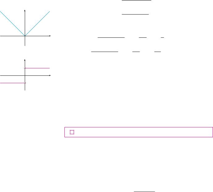
2.7EXERCISES

1.A curve has equation y ! f "x#.

(a)Write an expression for the slope of the secant line through the points P"3, f "3## and Q"x, f "x##.

(b)Write an expression for the slope of the tangent line at P.

;2. Graph the curve y ! ex in the viewing rectangles $"1, 1% by $0, 2%, $"0.5, 0.5% by $0.5, 1.5%, and $"0.1, 0.1% by $0.9, 1.1%. What do you notice about the curve as you zoom in toward the point "0, 1#?

3.(a) Find the slope of the tangent line to the parabola

y ! 4x " x2 at the point "1, 3#

(i) using Deﬁnition 1 (ii) using Equation 2

(b)Find an equation of the tangent line in part (a).

;(c) Graph the parabola and the tangent line. As a check on your work, zoom in toward the point "1, 3# until the parabola and the tangent line are indistinguishable.

4. (a) Find the slope of the tangent line to the curve y ! x " x3

at the point "1, 0#
(i) using Deﬁnition 1	(ii) using Equation 2

(b)Find an equation of the tangent line in part (a).

;(c) Graph the curve and the tangent line in successively smaller viewing rectangles centered at "1, 0# until the curve and the line appear to coincide.

5–8 Find an equation of the tangent line to the curve at the given point.

y !

x " 1

, "3, 2#

y ! 2x3 " 5x, ""1, 3#

x " 2

y ! sx , (1, 1#

y !

, "0, 0#

" x #

9. (a) Find the slope of the tangent to the curve

y ! 3 # 4x2 " 2x3 at the point where x ! a.

(b)Find equations of the tangent lines at the points "1, 5# and "2, 3#.

;(c) Graph the curve and both tangents on a common screen.

10.(a) Find the slope of the tangent to the curve y ! 1!sx at the point where x ! a.

(b)Find equations of the tangent lines at the points "1, 1# and (4, 12 ).

;(c) Graph the curve and both tangents on a common screen.

11.(a) A particle starts by moving to the right along a horizontal line; the graph of its position function is shown. When is the particle moving to the right? Moving to the left?

Standing still?

(b) Draw a graph of the velocity function.

s (meters)
4
2
0	2	4	6	t (seconds)

12.Shown are graphs of the position functions of two runners, A and B, who run a 100-m race and ﬁnish in a tie.

s (meters)
80		A
		A
40		B
		B
0	4	8	12	t (seconds)

(a)Describe and compare how the runners run the race.

(b)At what time is the distance between the runners the greatest?

(c)At what time do they have the same velocity?

13.If a ball is thrown into the air with a velocity of 40 ft!s, its height (in feet) after t seconds is given by y ! 40t " 16t2. Find the velocity when t ! 2.

14.If a rock is thrown upward on the planet Mars with a velocity of 10 m!s, its height (in meters) after t seconds is given by H ! 10t " 1.86t2.

(a)Find the velocity of the rock after one second.

(b)Find the velocity of the rock when t ! a.

(c)When will the rock hit the surface?

(d)With what velocity will the rock hit the surface?

15.The displacement (in meters) of a particle moving in a straight line is given by the equation of motion s ! 1!t2, where t is measured in seconds. Find the velocity of the particle at times t ! a, t ! 1, t ! 2, and t ! 3.

16.The displacement (in meters) of a particle moving in a straight line is given by s ! t2 " 8t # 18, where t is measured in seconds.

(a)Find the average velocity over each time interval:

(i)	$3, 4%	(ii)	$3.5, 4%
(iii)	$4, 5%	(iv)	$4, 4.5%

(b)Find the instantaneous velocity when t ! 4.

(c)Draw the graph of s as a function of t and draw the secant lines whose slopes are the average velocities in part (a) and the tangent line whose slope is the instantaneous velocity in part (b).

17.For the function t whose graph is given, arrange the following numbers in increasing order and explain your reasoning:

t)""2#

t)"0#

t)"2#

t)"4#

SECTION 2.7 DERIVATIVES AND RATES OF CHANGE |||| 151

y=©


		_		1	0	1		2			3			4			x

18.(a) Find an equation of the tangent line to the graph of y ! t"x# at x ! 5 if t"5# ! "3 and t)"5# ! 4.

(b)If the tangent line to y ! f "x# at (4, 3) passes through the point (0, 2), ﬁnd f "4# and f )"4#.

19. Sketch the graph of a function f for which f "0# ! 0, f )"0# ! 3, f )"1# ! 0, and f )"2# ! "1.

20.Sketch the graph of a function t for which t"0# ! t)"0# ! 0, t)""1# ! "1, t)"1# ! 3, and t)"2# ! 1.

21. If f "x# ! 3x2 " 5x, ﬁnd f )"2# and use it to ﬁnd an equation of the tangent line to the parabola y ! 3x2 " 5x at the point "2, 2#.

22.If t"x# ! 1 " x3, ﬁnd t)"0# and use it to ﬁnd an equation of the tangent line to the curve y ! 1 " x3 at the point "0, 1#.

23.(a) If F"x# ! 5x!"1 # x2#, ﬁnd F)"2# and use it to ﬁnd an

equation of the tangent line to the curve y ! 5x!"1 # x2# at the point "2, 2#.

;(b) Illustrate part (a) by graphing the curve and the tangent line on the same screen.

24.(a) If G"x# ! 4x2 " x3, ﬁnd G)"a# and use it to ﬁnd equations of the tangent lines to the curve y ! 4x2 " x3 at the points "2, 8# and "3, 9#.

;(b) Illustrate part (a) by graphing the curve and the tangent lines on the same screen.

25–30 Find f )"a#.
25.	f "x# ! 3 " 2x # 4x2				26.	f "t# ! t4 " 5t
27.	f "t# !	2t # 1			28.	f "x# !	x2 # 1
27.	f "t# !		t # 3		28.	f "x# !	x " 2
			t # 3				x " 2
		1
29.	f "x# !	1			30.	f "x# ! s3x # 1

			sx #	2
			sx #	2

31–36 Each limit represents the derivative of some function f at some number a. State such an f and a in each case.


31.	lim	"1 # h#10 " 1
31.	lim	h
	h l0	h
33.	lim	2x " 32
33.	lim	x " 5
	x l5	x " 5
35.	lim	cos"+ # h# # 1
	h l0	h

		4		16 # h	" 2
32.	lim		s
				h
	h l0
34.	lim tan x " 1
	x l +!4			x " +!4
36.	lim		t4	# t " 2
				t " 1
	t l1

152 |||| CHAPTER 2 LIMITS AND DERIVATIVES

37–38 A particle moves along a straight line with equation of motion s ! f !t", where s is measured in meters and t in seconds. Find the velocity and the speed when t ! 5.

37. f !t" ! 100 % 50t $ 4.9t2 38. f !t" ! t$1	$ t

39.A warm can of soda is placed in a cold refrigerator. Sketch the graph of the temperature of the soda as a function of time. Is the initial rate of change of temperature greater or less than the rate of change after an hour?

40.A roast turkey is taken from an oven when its temperature has reached 185°F and is placed on a table in a room where the temperature is 75°F. The graph shows how the temperature of the turkey decreases and eventually approaches room temperature. By measuring the slope of the tangent, estimate the rate of change of the temperature after an hour.

T (°F)
200
		P
100
0	30	60	90	120	150	t	(min)

41.The table shows the estimated percentage P of the population of Europe that use cell phones. (Midyear estimates are given.)

Year	1998	1999	2000	2001	2002	2003

P	28	39	55	68	77	83

(a) Find the average rate of cell phone growth
(i)	from 2000 to 2002		(ii)	from 2000 to 2001
(iii)	from 1999 to 2000

In each case, include the units.

(b) Estimate the instantaneous rate of growth in 2000 by taking the average of two average rates of change. What are its units?

42. The number N of locations of a popular coffeehouse chain is given in the table. (The numbers of locations as of June 30 are given.)

	Year	1998	1999		2000	2001	2002

	N	1886	2135		3501	4709	5886

(a) Find the average rate of growth
(i)	from 2000 to 2002			(ii)	from 2000 to 2001
(iii)	from 1999 to 2000

In each case, include the units.

(b)Estimate the instantaneous rate of growth in 2000 by taking the average of two average rates of change. What are its units?

(c)Estimate the instantaneous rate of growth in 2000 by measuring the slope of a tangent.

43.The cost (in dollars) of producing x units of a certain commodity is C!x" ! 5000 % 10x % 0.05x2.

(a)Find the average rate of change of C with respect to x when the production level is changed

(i)from x ! 100 to x ! 105

(ii)from x ! 100 to x ! 101

(b)Find the instantaneous rate of change of C with respect to x when x ! 100. (This is called the marginal cost.

Its signiﬁcance will be explained in Section 3.7.)

44.If a cylindrical tank holds 100,000 gallons of water, which can be drained from the bottom of the tank in an hour, then Torricelli’s Law gives the volume V of water remaining in the tank after t minutes as

V!t" ! 100,000#1	$	t	$2	0 # t # 60
		60

Find the rate at which the water is ﬂowing out of the tank (the instantaneous rate of change of V with respect to t) as a function of t. What are its units? For times t ! 0, 10, 20, 30, 40, 50, and 60 min, ﬁnd the ﬂow rate and the amount of water remaining in the tank. Summarize your ﬁndings in a sentence or two. At what time is the ﬂow rate the greatest? The least?

45.The cost of producing x ounces of gold from a new gold mine is C ! f !x" dollars.

(a)What is the meaning of the derivative f !!x"? What are its units?

(b)What does the statement f !!800" ! 17 mean?

(c)Do you think the values of f !!x" will increase or decrease in the short term? What about the long term? Explain.

46.The number of bacteria after t hours in a controlled laboratory experiment is n ! f !t".

(a)What is the meaning of the derivative f !!5"? What are its units?

(b)Suppose there is an unlimited amount of space and nutrients for the bacteria. Which do you think is larger,

f !!5" or f !!10"? If the supply of nutrients is limited, would that affect your conclusion? Explain.

47.Let T!t" be the temperature (in "F) in Dallas t hours after midnight on June 2, 2001. The table shows values of this function recorded every two hours. What is the meaning of T!!10"?

Estimate its value.

t	0	2	4	6	8	10	12	14

T	73	73	70	69	72	81	88	91

WRITING PROJECT EARLY METHODS FOR FINDING TANGENTS |||| 153

48.The quantity (in pounds) of a gourmet ground coffee that is sold by a coffee company at a price of p dollars per pound is Q ! f ! p".

(a)What is the meaning of the derivative f !!8"? What are its units?

(b)Is f !!8" positive or negative? Explain.

49.The quantity of oxygen that can dissolve in water depends on the temperature of the water. (So thermal pollution inﬂuences the oxygen content of water.) The graph shows how oxygen solubility S varies as a function of the water temperature T.

(a)What is the meaning of the derivative S!!T"? What are its units?

(b)Estimate the value of S!!16" and interpret it.

(mg/L)


0	8 16 24 32 40 T (°C)

Adapted from Environmental Science: Science: Living Within the

Reprinted by permission of Prentice-Hall, Inc., Upper Saddle River, NJ.

50.The graph shows the inﬂuence of the temperature T on the maximum sustainable swimming speed S of Coho salmon.

(a)What is the meaning of the derivative S!!T"? What are its units?

(b)Estimate the values of S!!15" and S!!25" and interpret them.

(cm/s)

T (°C)

51–52 Determine whether f !!0" exists.

x sin

x " 0

51.

f !x" ! %0

x ! 0

x2 sin

x " 0

52. f !x" ! %0

x ! 0

	W R I T I N G	E A R LY M E T H O D S F O R F I N D I N G TA N G E N T S
	P R O J E C T
	P R O J E C T	The ﬁrst person to formulate explicitly the ideas of limits and derivatives was Sir Isaac Newton in


		the 1660s. But Newton acknowledged that “If I have seen further than other men, it is because I
		have stood on the shoulders of giants.” Two of those giants were Pierre Fermat (1601–1665) and
		Newton’s teacher at Cambridge, Isaac Barrow (1630–1677). Newton was familiar with the meth-
		ods that these men used to ﬁnd tangent lines, and their methods played a role in Newton’s eventual
		formulation of calculus.
		The following references contain explanations of these methods. Read one or more of the
		references and write a report comparing the methods of either Fermat or Barrow to modern
		methods. In particular, use the method of Section 2.7 to ﬁnd an equation of the tangent line to the
		curve y ! x3 % 2x at the point (1, 3) and show how either Fermat or Barrow would have solved
		the same problem. Although you used derivatives and they did not, point out similarities between
		the methods.
		1. Carl Boyer and Uta Merzbach, A History of Mathematics (New York: Wiley, 1989),
		pp. 389, 432.
		2. C. H. Edwards, The Historical Development of the Calculus (New York: Springer-Verlag,
		1979), pp. 124, 132.
		3. Howard Eves, An Introduction to the History of Mathematics, 6th ed. (New York: Saunders,
		1990), pp. 391, 395.
		4. Morris Kline, Mathematical Thought from Ancient to Modern Times (New York:
		Oxford University Press, 1972), pp. 344, 346.

154 |||| CHAPTER 2 LIMITS AND DERIVATIVES

2 . 8 T H E D E R I VAT I V E A S A F U N C T I O N

In the preceding section we considered the derivative of a function f at a ﬁxed number a:

1	.f !!a" ! lim	f !a % h" $ f !a"
		h
	h l0

Here we change our point of view and let the number a vary. If we replace a in Equation 1 by a variable x, we obtain

2	f !!x" ! lim	f !x % h" $ f !x"
2	f !!x" ! lim	h
	h l0	h

Given any number x for which this limit exists, we assign to x the number f !!x". So we can regard f ! as a new function, called the derivative of f and deﬁned by Equation 2. We know that the value of f ! at x, f !!x", can be interpreted geometrically as the slope of the tangent line to the graph of f at the point !x, f !x"".

The function f ! is called the derivative of f because it has been “derived” from f by the limiting operation in Equation 2. The domain of f ! is the set (x ) f !!x" exists' and may be smaller than the domain of f.

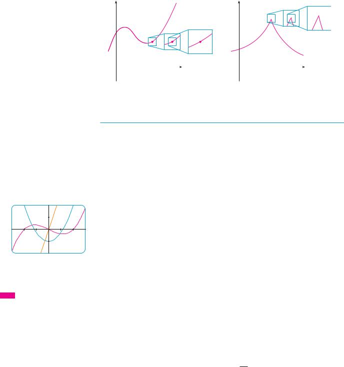
V EXAMPLE 1 The graph of a function f is given in Figure 1. Use it to sketch the graph of the derivative f !.

y=Ä

0	1	x
	1

FIGURE 1

SOLUTION We can estimate the value of the derivative at any value of x by drawing the tangent at the point !x, f !x"" and estimating its slope. For instance, for x ! 5 we draw the tangent at P in Figure 2(a) and estimate its slope to be about 32 , so f !!5" & 1.5. This allows us to plot the point P!!5, 1.5" on the graph of f ! directly beneath P. Repeating this procedure at several points, we get the graph shown in Figure 2(b). Notice that the tangents at A, B, and C are horizontal, so the derivative is 0 there and the graph of f ! crosses the x-axis at the points A!, B!, and C!, directly beneath A, B, and C. Between A and B the tangents have positive slope, so f !!x" is positive there. But between B and C the tangents have negative slope, so f !!x" is negative there.

SECTION 2.8 THE DERIVATIVE AS A FUNCTION

m=0

y=Ä

m•2

m=0

Visual 2.8 shows an animation of

TEC

Figure 2 for several functions.

(a)

y=f»(x)

P»(5,!1.5)

A»

B»

C»

||||155

FIGURE 2

(b)

V EXAMPLE 2

(a)If f !x" ! x3 $ x, ﬁnd a formula for f !!x".

(b)Illustrate by comparing the graphs of f and f !.

SOLUTION

(a) When using Equation 2 to compute a derivative, we must remember that the variable is h and that x is temporarily regarded as a constant during the calculation of the limit.

f !!x" ! lim

f !x % h" $ f !x"

! lim

*!x % h"3 $ !x % h"+ $ *x3

$ x+

h l0

! lim

% 3x2h % 3xh2

% h3

$ x $ h $ x3 % x

h l0

! lim

3x2h % 3xh2 % h3

$ h

! lim !3x2 % 3xh % h2

$ 1" ! 3x2

$ 1

h l0

156 |||| CHAPTER 2 LIMITS AND DERIVATIVES

(b) We use a graphing device to graph f and f ! in Figure 3. Notice that f !!x" ! 0 when f has horizontal tangents and f !!x" is positive when the tangents have positive slope. So these graphs serve as a check on our work in part (a).

f»

FIGURE 3

EXAMPLE 3 If f !x" ! sx , ﬁnd the derivative of f. State the domain of f !.

SOLUTION

f !!x" ! lim

f !x % h" $ f !x"

! lim

sx % h $ sx

h l0

Here we rationalize the numerator.

! lim

sx % h $ sx

sx % h % sx

h l0

sx % h % sx $

! lim

!x % h" $ x

! lim

h(sx % h % sx )

sx % h % sx

h l0

sx % sx

2sx

We see that f !!x" exists if x ' 0, so the domain of f ! is !0, &". This is smaller than the

domain of f , which is *0, &".

(a) Ä=Ïxã

Let’s check to see that the result of Example 3 is reasonable by looking at the graphs of

and f ! in Figure 4. When x is close to 0, sx is also close to 0, so f !!x" ! 1,(2sx ) is

very large and this corresponds to the steep tangent lines near !0, 0" in Figure 4(a) and the

large values of f !!x" just to the right of 0 in Figure 4(b). When x is large, f !!x" is very small

and this corresponds to the ﬂatter tangent lines at the far right of the graph of f and the

horizontal asymptote of the graph of f !.

EXAMPLE 4 Find f ! if f !x" !

1 $ x

(b) f»(x)=

2 % x

Ïãx

FIGURE 4

SOLUTION

1 $ !x % h"

1 $ x

f !!x" ! lim

f !x % h" $ f !x"

! lim

2 % !x % h"

2 % x

h l0

! lim

!1 $ x $ h"!2 % x" $ !1

$ x"!2 % x % h"

ad $ bc

h!2 % x % h"!2 % x"

h l0

! lim

h l0

! lim

h l0

!2 $ x $ 2h $ x2 $ xh" $ !2 $ x % h $ x2 $ xh"

h!2 % x % h"!2 % x"

$3h	! lim	$3	! $	3		M
h!2 % x % h"!2 % x"		!2 % x % h"!2 % x"		!2 % x"	2
	h l0

LEIBNIZ

Gottfried Wilhelm Leibniz was born in Leipzig in 1646 and studied law, theology, philosophy, and mathematics at the university there, graduating with a bachelor’s degree at age 17. After earning his doctorate in law at age 20, Leibniz

entered the diplomatic service and spent most of his life traveling to the capitals of Europe on political missions. In particular, he worked to avert a French military threat against Germany and attempted to reconcile the Catholic and Protestant churches.

His serious study of mathematics did not begin until 1672 while he was on a diplomatic mission in Paris. There he built a calculating machine and met scientists, like Huygens, who directed his attention to the latest developments in mathematics and science. Leibniz sought to develop a symbolic logic and system of notation that would simplify logical reasoning. In particular, the version of calculus that he published in 1684 established the notation and the rules for ﬁnding derivatives that we use today.

Unfortunately, a dreadful priority dispute arose in the 1690s between the followers of Newton and those of Leibniz as to who had invented calculus ﬁrst. Leibniz was even accused of plagiarism by members of the Royal Society in England. The truth is that each man invented calculus independently. Newton arrived at his version of calculus ﬁrst but, because of his fear of controversy, did not publish it immediately. So Leibniz’s 1684 account of calculus was the ﬁrst to be published.

SECTION 2.8 THE DERIVATIVE AS A FUNCTION |||| 157

OT H E R N OTAT I O N S

If we use the traditional notation y ! f !x" to indicate that the independent variable is x and the dependent variable is y, then some common alternative notations for the derivative are as follows:

f !!x" ! y! ! dy	!	df	!	d	f !x" ! Df !x" ! Dx f !x"
		dx		dx
dx

The symbols D and d,dx are called differentiation operators because they indicate the operation of differentiation, which is the process of calculating a derivative.

The symbol dy,dx, which was introduced by Leibniz, should not be regarded as a ratio (for the time being); it is simply a synonym for f !!x". Nonetheless, it is a very useful and suggestive notation, especially when used in conjunction with increment notation. Referring to Equation 2.7.6, we can rewrite the deﬁnition of derivative in Leibniz notation in the form

dy ! lim )y dx )x l0 )x

If we want to indicate the value of a derivative dy,dx in Leibniz notation at a speciﬁc number a, we use the notation

		dy			or		dy
		dx .x!a			or		dx -x!a
		dx .x!a					dx -x!a
which is a synonym for f !!a".

	3	DEFINITION A function	f is differentiable at a if							f !!a" exists. It is differen-
	tiable on an open interval !a, b" [or !a, &" or !$&, a" or !$&, &"] if it is differ-
	entiable at every number in the interval.

	EXAMPLE 5 Where is the function f !x" ! ) x ) differentiable?
V

SOLUTION		If x ' 0, then ) x ) ! x and we can choose h small enough that x % h ' 0 and
hence ) x % h ) ! x % h. Therefore, for x ' 0, we have
		f !!x" ! lim		) x % h ) $ ) x )
		f !!x" ! lim
		h l0		h
		! lim		!x % h" $ x		! lim		h	! lim 1 ! 1
		! lim		h		! lim			! lim 1 ! 1
		h l0		h			h l0	h		h l0

and so f is differentiable for any x ' 0.

Similarly, for x ( 0 we have ) x ) ! $x and h can be chosen small enough that x % h ( 0 and so ) x % h ) ! $!x % h". Therefore, for x ( 0,

f !!x" ! lim	) x % h )	$ ) x )
	h
h l0
! lim	$!x % h" $ !$x"
		h
h l0

and so f is differentiable for any x ( 0.

! lim	$h	! lim !$1" ! $1
	h
h l0		h l0

P R O O F

158 |||| CHAPTER 2 LIMITS AND DERIVATIVES

		For x ! 0 we have to investigate
				f !!0" ! lim	f !0 % h" $ f !0"
				h l0		h
y				! lim	) 0 % h ) $ ) 0 )				!if it exists"
				! lim	) 0 % h ) $ ) 0 )				!if it exists"
				h l0		h
		Let’s compute the left and right limits separately:
0	x		lim	) 0 % h ) $ ) 0 ) ! lim			) h )	! lim		h	! lim 1 ! 1
0			h l0%	h	h l0%		h	h l0%		h	h l0%
(a) y=Ä=\| x \|		and	lim ) 0 % h ) $ ) 0 ) ! lim			) h )	! lim		$h	! lim !$1" ! $1
			h l0$	h	h l0$	h	h l0$		h		h l0$
y		Since these limits are different, f !!0" does not exist. Thus f									is differentiable at all x
											is differentiable at all x
1		except 0.
0		A formula for f ! is given by
0	x					1	if	x ' 0
_1						1	if	x ' 0
_1				f !!x" ! %$1 if x ( 0
				f !!x" ! %$1 if x ( 0

(b) y=f»(x)

FIGURE 5

and its graph is shown in Figure 5(b). The fact that f !!0" does not exist is reﬂected geometrically in the fact that the curve y ! ) x ) does not have a tangent line at !0, 0". [See Figure 5(a).] M

Both continuity and differentiability are desirable properties for a function to have. The following theorem shows how these properties are related.

THEOREM If f is differentiable at a, then f is continuous at a.

To prove that f is continuous at a, we have to show that limx la f !x" ! f !a". We do this by showing that the difference f !x" $ f !a" approaches 0.

The given information is that f is differentiable at a, that is,

	f !!a" ! lim	f !x" $ f !a"
	f !!a" ! lim	x $ a
	x la	x $ a

exists (see Equation 2.7.5). To connect the given and the unknown, we divide and multiply f !x" $ f !a" by x $ a (which we can do when x " a):

f !x" $ f !a" ! f !x" $ f !a" !x $ a" x $ a

Thus, using the Product Law and (2.7.5), we can write

lim * f !x" $ f !a"+ ! lim		f !x" $ f !a"	!x $ a"
lim * f !x" $ f !a"+ ! lim		x $ a	!x $ a"
x la	x la	x $ a
	! lim	f !x" $ f !a"	! lim !x $ a"
	! lim	x $ a	! lim !x $ a"
	x la	x $ a	x la

! f !!a" ! 0 ! 0

y	vertical tangent
	vertical tangent
	line
0	a	x

FIGURE 6

SECTION 2.8 THE DERIVATIVE AS A FUNCTION |||| 159

To use what we have just proved, we start with f !x" and add and subtract f !a": lim f !x" ! lim * f !a" % ! f !x" $ f !a""+

x la

! lim f !a" % lim * f !x" $ f !a"+

x la x la

! f !a" % 0 ! f !a"

Therefore f is continuous at a. M

\|		The converse of Theorem 4 is false; that is, there are functions that are continuous
\|	N OT E
	but not	differentiable. For instance, the function f !x" ! ) x )						is continuous at 0 because
		lim f !x" ! lim		)	x	)	! 0 ! f !0"
		x l0	x l0	)		)

(See Example 7 in Section 2.3.) But in Example 5 we showed that f is not differentiable at 0.

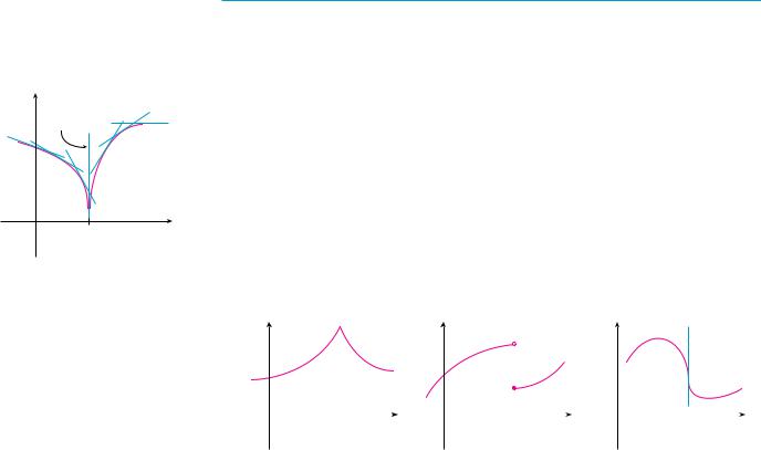
H OW C A N A F U N C T I O N FA I L TO B E D I F F E R E N T I A B L E ?

We saw that the function y ! ) x ) in Example 5 is not differentiable at 0 and Figure 5(a) shows that its graph changes direction abruptly when x ! 0. In general, if the graph of a function f has a “corner” or “kink” in it, then the graph of f has no tangent at this point and f is not differentiable there. [In trying to compute f !!a", we ﬁnd that the left and right limits are different.]

Theorem 4 gives another way for a function not to have a derivative. It says that if f is not continuous at a, then f is not differentiable at a. So at any discontinuity (for instance, a jump discontinuity) f fails to be differentiable.

A third possibility is that the curve has a vertical tangent line when x ! a; that is, f is continuous at a and

lim ) f !!x" ) ! &

x la

This means that the tangent lines become steeper and steeper as x l a. Figure 6 shows one way that this can happen; Figure 7(c) shows another. Figure 7 illustrates the three possibilities that we have discussed.

FIGURE 7

Three ways for ƒ not to be differentiable at a

(a) A corner

(b) A discontinuity

A graphing calculator or computer provides another way of looking at differentiability. If f is differentiable at a, then when we zoom in toward the point !a, f !a"" the graph

160 |||| CHAPTER 2 LIMITS AND DERIVATIVES

	2
	f ·	fª	f
		fª

_1.5			1.5
	_2

FIGURE 10

TEC In Module 2.8 you can see how changing the coefﬁcients of a polynomial f affects the appearance of the graphs of f , f !, and f ".

straightens out and appears more and more like a line. (See Figure 8. We saw a speciﬁc example of this in Figure 2 in Section 2.7.) But no matter how much we zoom in toward a point like the ones in Figures 6 and 7(a), we can’t eliminate the sharp point or corner (see Figure 9).

	0		x	0		x
		a			a
FIGURE 8				FIGURE 9
ƒ is differentiable at a.				ƒ is not differentiable at a.

HIGHER DERIVATIVES

If f is a differentiable function, then its derivative f ! is also a function, so f ! may have a derivative of its own, denoted by ! f !"! ! f ". This new function f " is called the second derivative of f because it is the derivative of the derivative of f. Using Leibniz notation, we write the second derivative of y ! f !x" as

d	%	dy	& !	d2y
dx	%	dx	& !	dx2

EXAMPLE 6 If f !x" ! x3 $ x, ﬁnd and interpret f "!x".

SOLUTION In Example 2 we found that the ﬁrst derivative is f !!x" ! 3x2 $ 1. So the second derivative is

f !!!x" ! ! f !"!!x"

! lim

f !!x # h" $ f !!x"

! lim

#3!x # h"2

$ 1$ $ #3x2

$ 1$

h l0

! lim

3x2

# 6xh # 3h2

$ 1

$ 3x2

# 1

! lim

!6x #

3h" ! 6x

h l0

The graphs of f , f !, f " are shown in Figure 10.
We can interpret f "!x" as the slope of the curve y ! f !!x" at the point !x, f !!x"". In
other words, it is the rate of change of the slope of the original curve y ! f !x".
Notice from Figure 10 that f "!x" is negative when y ! f !!x" has negative slope
and positive when y ! f !!x" has positive slope. So the graphs serve as a check on our
calculations.	M

In general, we can interpret a second derivative as a rate of change of a rate of change. The most familiar example of this is acceleration, which we deﬁne as follows.

If s ! s!t" is the position function of an object that moves in a straight line, we know that its ﬁrst derivative represents the velocity v!t" of the object as a function of time:

v!t" ! s!!t" ! dsdt

SECTION 2.8 THE DERIVATIVE AS A FUNCTION |||| 161

The instantaneous rate of change of velocity with respect to time is called the acceleration a!t" of the object. Thus the acceleration function is the derivative of the velocity function and is therefore the second derivative of the position function:

a!t" ! v!!t" ! s"!t"

or, in Leibniz notation,
a !	dv	!	d2s
	dt		dt2

The third derivative f % is the derivative of the second derivative: f % ! ! f ""!. So f %!x" can be interpreted as the slope of the curve y ! f "!x" or as the rate of change of f "!x". If y ! f !x", then alternative notations for the third derivative are

y% ! f %!x" !	d	%	d2 y	& !	d3y
	dx		dx2		dx3

The process can be continued. The fourth derivative f " is usually denoted by f !4". In general, the nth derivative of f is denoted by f !n" and is obtained from f by differentiating n times. If y ! f !x", we write

y!n" ! f !n"!x" ! dn y dxn

EXAMPLE 7 If f !x" ! x3 $ x, ﬁnd f %!x" and f !4"!x".

SOLUTION In Example 6 we found that f "!x" ! 6x. The graph of the second derivative has equation y ! 6x and so it is a straight line with slope 6. Since the derivative f %!x" is the slope of f "!x", we have

f %!x" ! 6

for all values of x. So f % is a constant function and its graph is a horizontal line. Therefore, for all values of x,

f !4"!x" ! 0

We can interpret the third derivative physically in the case where the function is the position function s ! s!t" of an object that moves along a straight line. Because s% ! !s""! ! a!, the third derivative of the position function is the derivative of the acceleration function and is called the jerk:

j !	da	!	d3s
	dt		dt3

Thus the jerk j is the rate of change of acceleration. It is aptly named because a large jerk means a sudden change in acceleration, which causes an abrupt movement in a vehicle.

We have seen that one application of second and third derivatives occurs in analyzing the motion of objects using acceleration and jerk. We will investigate another application of second derivatives in Section 4.3, where we show how knowledge of f " gives us information about the shape of the graph of f. In Chapter 11 we will see how second and higher derivatives enable us to represent functions as sums of inﬁnite series.

162|||| CHAPTER 2 LIMITS AND DERIVATIVES

2.8EXERCISES

1–2 Use the given graph to estimate the value of each derivative. Then sketch the graph of f !.

1.	(a)	f !!$3"	y
	(b)	f !!$2"	y=f(x)
	(c)	f !!$1"		1
	(d)	f !!0"		1
	(d)	f !!0"	0		x
	(e)	f !!1"	0	1	x

(f)f !!2"

(g)f !!3"

2.	(a)	f !!0"	y
	(b)	f !!1"		y=f(x)
	(c) f !!2"
	(d) f !!3"
	(e) f !!4"		1
	(f)	f !!5"	1
	(f)	f !!5"	0	1	x
			0	1	x
3. Match the graph of each function in (a)–(d) with the graph of
	its derivative in I–IV. Give reasons for your choices.

(a)y

0 x

(c)y

0 x

I y

0 x

III y

0 x

(b)	y
	0	x
(d)	y
	0	x
II	y
	0	x

IV	y
	0	x

4 –11 Trace or copy the graph of the given function f . (Assume that the axes have equal scales.) Then use the method of Example 1 to sketch the graph of f ! below it.

4.y

0 x

	0	x	0	x
			0	x
7.	y	8.	y
	0	x	0	x
9.	y	10.	y
	0	x	0	x
			0	x
11.	y

12.Shown is the graph of the population function P!t" for yeast cells in a laboratory culture. Use the method of Example 1 to

P(yeast cells)

500

0
	5		10		15 t (hours)

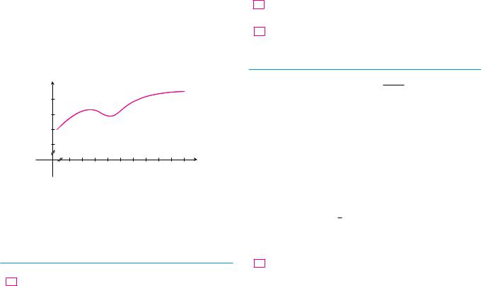
graph the derivative P!!t". What does the graph of P! tell us about the yeast population?

13.The graph shows how the average age of ﬁrst marriage of Japanese men has varied in the last half of the 20th century. Sketch the graph of the derivative function M!!t". During which years was the derivative negative?

M
27
25
1960 1970 1980 1990	2000 t
14 –16 Make a careful sketch of the graph of f	and below it

sketch the graph of f ! in the same manner as in Exercises 4–11. Can you guess a formula for f !!x" from its graph?

14. f !x" ! sin x 15. f !x" ! ex

16.f !x" ! ln x

;17. Let f !x" ! x2.

(a)Estimate the values of f !!0", f !(12 ), f !!1", and f !!2" by using a graphing device to zoom in on the graph of f.

(b)Use symmetry to deduce the values of f !($12 ), f !!$1", and f !!$2".

(c)Use the results from parts (a) and (b) to guess a formula for f !!x".

(d)Use the deﬁnition of a derivative to prove that your guess in part (c) is correct.

;18. Let f !x" ! x3.

(a)Estimate the values of f !!0", f !(12 ), f !!1", f !!2", and f !!3" by using a graphing device to zoom in on the graph of f.

(b)Use symmetry to deduce the values of f !($12 ), f !!$1", f !!$2", and f !!$3".

(c)Use the values from parts (a) and (b) to graph f !.

(d)Guess a formula for f !!x".

(e)Use the deﬁnition of a derivative to prove that your guess in part (d) is correct.

19–29 Find the derivative of the function using the deﬁnition of derivative. State the domain of the function and the domain of its derivative.

19.	f !x" ! 21 x $ 31	20.	f !x" ! mx # b
21.	f !t" ! 5t $ 9t2	22.	f !x" ! 1.5x2 $ x # 3.7
23.	f !x" ! x3 $ 3x # 5	24.	f !x" ! x # s
				x

SECTION 2.8 THE DERIVATIVE AS A FUNCTION |||| 163

							3 # x
25.	t!x" ! s1 #						3 # x
25.				2x	26.	f !x" ! 1 $ 3x
				2x	26.	f !x" ! 1 $ 3x
27.		4t				1

	G!t" ! t #		1		28.	t!t" ! st
	G!t" ! t #		1		28.	t!t" ! st

29.f !x" ! x4

30.(a) Sketch the graph of f !x" ! s6 $ x by starting with the graph of y ! sx and using the transformations of Section 1.3.

(b)Use the graph from part (a) to sketch the graph of f !.

(c)Use the deﬁnition of a derivative to ﬁnd f !!x". What are the domains of f and f !?

;(d) Use a graphing device to graph f ! and compare with your sketch in part (b).

31.(a) If f !x" ! x4 # 2x, ﬁnd f !!x".

;(b) Check to see that your answer to part (a) is reasonable by comparing the graphs of f and f !.

32.(a) If f !t" ! t2 $ st , ﬁnd f !!t".

;(b) Check to see that your answer to part (a) is reasonable by comparing the graphs of f and f !.

33.The unemployment rate U!t" varies with time. The table (from the Bureau of Labor Statistics) gives the percentage of unemployed in the US labor force from 1993 to 2002.

t	U!t"	t	U!t"

1993	6.9	1998	4.5
1994	6.1	1999	4.2
1995	5.6	2000	4.0
1996	5.4	2001	4.7
1997	4.9	2002	5.8

(a)What is the meaning of U!!t"? What are its units?

(b)Construct a table of values for U!!t".

34.Let P!t" be the percentage of Americans under the age of 18 at time t. The table gives values of this function in census years from 1950 to 2000.

t	P!t"	t	P!t"

1950	31.1	1980	28.0
1960	35.7	1990	25.7
1970	34.0	2000	25.7

(a)What is the meaning of P!!t"? What are its units?

(b)Construct a table of estimated values for P!!t".

(c)Graph P and P!.

(d)How would it be possible to get more accurate values for P!!t"?

164 |||| CHAPTER 2 LIMITS AND DERIVATIVES

35–38 The graph of f is given. State, with reasons, the numbers at which f is not differentiable.

35.	y			36.	y
	_2 0	2	x		0	2	4	x
	_2 0	2	x			2	4	x
37.	y			38.		y
_2	0	4	x		_2	0	2	x

;39. Graph the function f !x" ! x # s( x ( . Zoom in repeatedly, ﬁrst toward the point ($1, 0) and then toward the origin. What is different about the behavior of f in the vicinity of these two points? What do you conclude about the differentiability of f ?

;40. Zoom in toward the points (1, 0), (0, 1), and ($1, 0) on the graph of the function t!x" ! !x2 $ 1"2'3. What do you notice? Account for what you see in terms of the differentiability of t.

41.The ﬁgure shows the graphs of f , f !, and f ". Identify each curve, and explain your choices.

y a

42.The ﬁgure shows graphs of f, f !, f ", and f %. Identify each curve, and explain your choices.

y	a b c d

43.The ﬁgure shows the graphs of three functions. One is the position function of a car, one is the velocity of the car, and one is its acceleration. Identify each curve, and explain your choices.

y a

b c

44.The ﬁgure shows the graphs of four functions. One is the position function of a car, one is the velocity of the car, one is its acceleration, and one is its jerk. Identify each curve, and explain your choices.

a	d
b	c

0 t

;45– 46 Use the deﬁnition of a derivative to ﬁnd f !!x" and f "!x". Then graph f , f !, and f " on a common screen and check to see if your answers are reasonable.

45. f !x" ! 1 # 4x $ x2	46. f !x" ! 1'x

;47. If f !x" ! 2x2 $ x3, ﬁnd f !!x", f "!x", f %!x", and f !4"!x". Graph f , f !, f ", and f % on a common screen. Are the graphs consistent with the geometric interpretations of these derivatives?

48.(a) The graph of a position function of a car is shown, where s is measured in feet and t in seconds. Use it to graph the velocity and acceleration of the car. What is the acceleration at t ! 10 seconds?

100


0	10			20			t

(b)Use the acceleration curve from part (a) to estimate the jerk at t ! 10 seconds. What are the units for jerk?

<<< < Предыдущая 4 5 6 7 8 9 10 11 12 13 14 1516 / 9116 17 18 19 20 21 22 23 24 25 26 27 28 > Следующая >>>

Соседние файлы в предмете [НЕСОРТИРОВАННОЕ]

#
05.02.202055.36 Mб19Calculus, 7th Edition ( PDFDrive.com ).pdf
#
30.12.201945.82 Mб41Complete Solutions Manual for_ SINGLE VARIABLE CALCULUS Early Transcendentals 7th Edition by Stewart ( PDFDrive.com ).pdf
#
30.12.201918.09 Mб36[James_Stewart]_Single_Variable_Calculus_Early_Tr(BookFi).pdf