AREAS BETWEEN CURVES

Добавил:

PavelEngineer Опубликованный материал нарушает ваши авторские права? Сообщите нам.

Вуз:

Севастопольский Государственный Университет

Предмет:

[НЕСОРТИРОВАННОЕ]

Файл:

[James_Stewart]_Single_Variable_Calculus_Early_Tr(BookFi).pdf

Скачиваний:

Добавлен:

30.12.2019

Размер:

18.09 Mб

Скачать

☆

<<< < Предыдущая 28 29 30 31 32 33 34 35 36 37 38 3940 / 9140 41 42 43 44 45 46 47 48 49 50 51 52 > Следующая >>>

6.1

y=ƒ

0 a

y=©

FIGURE 1

S=s(x,y)|a¯x¯b, ©¯y¯ƒd

2x 2 dx 2 y0

In Chapter 5 we deﬁned and calculated areas of regions that lie under the graphs of functions. Here we use integrals to ﬁnd areas of regions that lie between the graphs of two functions.

Consider the region S that lies between two curves y f x and y t x and between the vertical lines x a and x b, where f and t are continuous functions and f x t x for all x in a, b . (See Figure 1.)

Just as we did for areas under curves in Section 5.1, we divide S into n strips of equal width and then we approximate the ith strip by a rectangle with base x and height f x*i t x*i . (See Figure 2. If we like, we could take all of the sample points to be right endpoints, in which case x*i xi.) The Riemann sum

f x*i t x*i x

i 1

is therefore an approximation to what we intuitively think of as the area of S.

y y

f(x*i )

f(x*i )-g(x*i )

_g(x*i )

x*i

0 a

Îx

FIGURE 2

(a) Typical rectangle

(b) Approximating rectangles

This approximation appears to become better and better as n l . Therefore we deﬁne the area A of the region S as the limiting value of the sum of the areas of these approximating rectangles.

1 A lim f x*i t x*i x

n l i 1

We recognize the limit in (1) as the deﬁnite integral of f t. Therefore we have the following formula for area.

2 The area A of the region bounded by the curves y f x , y t x , and the lines x a, x b, where f and t are continuous and f x t x for all x in a, b , is

A yb f x t x dx

Notice that in the special case where t x 0, S is the region under the graph of f and our general deﬁnition of area (1) reduces to our previous deﬁnition (Deﬁnition 2 in Section 5.1).

415

416 |||| CHAPTER 6 APPLICATIONS OF INTEGRATION

y						In the case where both f and tare positive, you can see from Figure 3 why (2) is true:
					y=ƒ	A area under y f x area under y t x
					y=ƒ
			S			b	b	b
						b	b	b
				y=©		ya	f x dx ya	t x dx ya f x t x dx
0		a			b x	EXAMPLE 1 Find the area of the region bounded above by y e x, bounded below by
FIGURE 3						y x, and bounded on the sides by x 0 and x 1.
FIGURE 3
	j	b		j	b	SOLUTION The region is shown in Figure 4. The upper boundary curve is y e			x	and the
A=		b			b					and the
A=			ƒ dx-		© dx	lower boundary curve is y x. So we use the area formula (2) with f x e x, t x x,

a 0, and b 1:

x=1

0	1	x
	1

FIGURE 4

		yT
				yT-yB
		yB	Îx
			Îx
0	a		b	x
	a		b

1	e x x dx e x 21 x 2]10
A y0	e x x dx e x 21 x 2]10
e 21 1 e 1.5		M

In Figure 4 we drew a typical approximating rectangle with width x as a reminder of the procedure by which the area is deﬁned in (1). In general, when we set up an integral for an area, it’s helpful to sketch the region to identify the top curve yT, the bottom curve yB, and a typical approximating rectangle as in Figure 5. Then the area of a typical rectangle is yT yB x and the equation

	n	b yT yB dx
A lim	yT yB x	b yT yB dx
n l i 1		ya

summarizes the procedure of adding (in a limiting sense) the areas of all the typical rectangles.

Notice that in Figure 5 the left-hand boundary reduces to a point, whereas in Figure 3 the right-hand boundary reduces to a point. In the next example both of the side boundaries reduce to a point, so the ﬁrst step is to ﬁnd a and b.

V EXAMPLE 2 Find the area of the region enclosed by the parabolas y x 2 and

y 2x x 2.

FIGURE 5

yT =2x- ≈

(1, 1)

yB	≈
Îx
(0, 0)	x

SOLUTION We ﬁrst ﬁnd the points of intersection of the parabolas by solving their equations simultaneously. This gives x 2 2x x 2, or 2x 2 2x 0. Thus 2x x 1 0, so x 0 or 1. The points of intersection are 0, 0 and 1, 1 .

We see from Figure 6 that the top and bottom boundaries are

yT 2x x 2 and yB x 2

The area of a typical rectangle is

yT yB x 2x x 2 x 2 x

and the region lies between x 0 and x 1. So the total area is

1.5
y=	x
	œ„„„„„≈+1
_1	2
	y=x$-x
_1

FIGURE 7

	√ (mi/h)
60			A
50			A
50
40
30				B
20
10
0	2	4	6	8	10	12	14	16	t
							(seconds)

FIGURE 8

SECTION 6.1 AREAS BETWEEN CURVES |||| 417

Sometimes it’s difﬁcult, or even impossible, to ﬁnd the points of intersection of two curves exactly. As shown in the following example, we can use a graphing calculator or computer to ﬁnd approximate values for the intersection points and then proceed as before.

EXAMPLE 3 Find the approximate area of the region bounded by the curves y x sx 2 1 and y x 4 x.

SOLUTION If we were to try to ﬁnd the exact intersection points, we would have to solve the equation

sx 2 1 x 4 x

This looks like a very difﬁcult equation to solve exactly (in fact, it’s impossible), so instead we use a graphing device to draw the graphs of the two curves in Figure 7. One intersection point is the origin. We zoom in toward the other point of intersection and ﬁnd that x 1.18. (If greater accuracy is required, we could use Newton’s method or a rootﬁnder, if available on our graphing device.) Thus an approximation to the area between the curves is

A	1.18		x 2x 1 x 4 x dx
A	0		x 2x 1 x 4 x dx
	y	s
	y	s

To integrate the ﬁrst term we use the subsitution u x 2 1. Then du 2x dx, and when x 1.18, we have u 2.39. So

2.39				du		1.18
A 21 y1						y0			x 4 x dx
				s
				s	u
												1.18
s			]12.39				x 5			x 2	0
		u					x 5			x 2
		u					5			2
s				1				1.18 5					1.18 2
	2.39							1.18 5					1.18 2
	2.39
									5			2
0.785														M

EXAMPLE 4 Figure 8 shows velocity curves for two cars, A and B, that start side by side and move along the same road. What does the area between the curves represent? Use the Midpoint Rule to estimate it.

SOLUTION We know from Section 5.4 that the area under the velocity curve A represents the distance traveled by car A during the ﬁrst 16 seconds. Similarly, the area under curve B is the distance traveled by car B during that time period. So the area between these curves, which is the difference of the areas under the curves, is the distance between the

cars after 16 seconds. We read the velocities from the graph and convert them to feet per second 1 mi h 52803600 ft s .

t	0	2	4	6	8	10	12	14	16

vA	0	34	54	67	76	84	89	92	95

vB	0	21	34	44	51	56	60	63	65

vA vB	0	13	20	23	25	28	29	29	30

418 |||| CHAPTER 6 APPLICATIONS OF INTEGRATION

We use the Midpoint Rule with n 4 intervals, so that t 4. The midpoints of the intervals are t1 2, t2 6, t3 10, and t4 14. We estimate the distance between the cars after 16 seconds as follows:

vB dt

t 13 23 28 29

4 93 372 ft

If we are asked to ﬁnd the area between the curves y f x

and y t x where

y=©

f x t x for some values of x but t x f x for other values of x, then we split the

S¡

S™

S£

given region S into several regions S1, S2, . . . with areas A1, A2, . . . as shown in Figure 9.

We then deﬁne the area of the region S to be the sum of the areas of the smaller regions

y=ƒ

S1, S2, . . . , that is, A A1 A2 . Since

f x t x

when f x t x

FIGURE 9

f x t x t x f x

when t x f x

we have the following expression for A.

The area between the curves y f x and y t x and between x a and

x b is

A yab f x t x dx

When evaluating the integral in (3), however, we must still split it into integrals corre-

sponding to A1, A2, . . . .

EXAMPLE 5 Find the area of the region bounded by the curves y sin x, y cos x,

x 0, and x 2.

SOLUTION

The points of intersection occur when sin x cos x, that is, when x 4

y =cos x

y=sin x

(since 0 x 2). The region is sketched in Figure 10. Observe that cos x sin x

when 0

4 but sin x cos x when

4 x

2. Therefore the required

A¡

A™

area is

x=π2

cos x sin x dx A1 A2

x=0

A y0

cos x sin x dx y 4

sin x cos x dx

[ cos x

[sin x cos x]0

sin x] 4

FIGURE 10

0 1 0 1

In this particular example we could have saved some work by noticing that the region

is symmetric about x

4 and so

A 2A1 2 y 4 cos x sin x dx

		y	(5, 4)
		4	(5, 4)
		4
x =1		¥-3
L	2
			xR=y+1
		0	x
(_1, _2)			_2

FIGURE 13

		y
y=œ„„„„„2x+6			(5,4)
			(5,4)
			A™
			y=x-1
3	A¡	0	x
			(_1, _2)
y=_œ„„„„„2x+6

FIGURE 14

SECTION 6.1 AREAS BETWEEN CURVES |||| 419

Some regions are best treated by regarding x as a function of y. If a region is bounded by curves with equations x f y , x t y , y c, and y d, where f and tare continuous and f y t y for c y d (see Figure 11), then its area is

A yd f y t y dy

y=d

Îy

x=g(y) x=f(y)

c	y=c
	y=c
0	x

xL xR

		Îy
	xR-xL
c
c
0		x

FIGURE 11

FIGURE 12

If we write xR for the right boundary and xL for the left boundary, then, as Figure 12 illustrates, we have

A yd xR xL dy

Here a typical approximating rectangle has dimensions xR xL and y.

V EXAMPLE 6 Find the area enclosed by the line y x 1 and the parabola

y 2 2x 6.

SOLUTION By solving the two equations we ﬁnd that the points of intersection are1, 2 and 5, 4 . We solve the equation of the parabola for x and notice from Figure 13 that the left and right boundary curves are

xL 21 y 2 3

xR y 1

We must integrate between the appropriate y-values, y 2 and y 4. Thus

A y42 xR xL dy

y42 [ y 1 (21 y 2 3)] dy
y42 ( 21 y 2 y 4) dy
	1		y 3	y	2		4
						4y
	2	3		2			2


61 64 8 16 (34 2 8) 18								M

We could have found the area in Example 6 by integrating with respect to x instead of y, but the calculation is much more involved. It would have meant splitting the region in two and computing the areas labeled A1 and A2 in Figure 14. The method we used in Example 6 is much easier.

420 |||| CHAPTER 6 APPLICATIONS OF INTEGRATION

6.1E X E R C I S E S

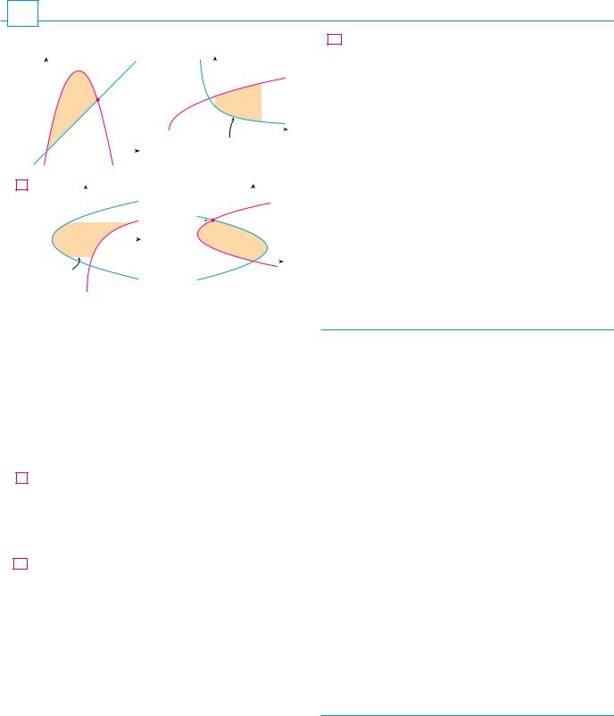
1– 4 Find the area of the shaded region.

y=5x-≈

y=œ„„„„x+2

(4,4)

x=2

y=x

x+1

x=¥-4y

x=¥-2

y=1

(_3,3)

x=ey

y=_1

x=2y-¥

21.	x 1 y 2,	x y 2 1
22.	y sin x 2 , y x
23.	y cos x,	y sin 2x, x 0, x 2
24.	y cos x,	y 1 cos x, 0 x

25.y x 2, y 2 x 2 1

26.y x , y x2 2

27. y 1 x,	y x,	y 41 x, x 0
28. y 3x 2,	y 8x 2,	4x y 4, x 0

29–30 Use calculus to ﬁnd the area of the triangle with the given vertices.

	0,	0 ,	2,	1 ,	1,	6
29.
30. 0,		5 ,	2,	2 ,	5,	1

5–28 Sketch the region enclosed by the given curves. Decide whether to integrate with respect to x or y. Draw a typical approximating rectangle and label its height and width. Then ﬁnd the area of the region.


5.	y x 1, y 9 x 2, x 1, x 2
6.	y sin x,				y e x, x 0,		x 2
7.	y x, y x 2
8.	y x 2 2x, y x 4
9.	y 1 x, y 1 x 2, x 2
10.	y 1 s					, y 3 x 3
					x
11.	y x 2,			y 2 x
12.	y x 2,			y 4x x 2
13.	y 12 x 2, y x 2 6
14. y cos x,					y 2 cos x,		0 x 2
15. y tan x,					y 2 sin x, 3 x 3
16.	y x 3 x, y 3x
17.	y s		,	y 21 x, x 9
		x
18.	y 8 x 2, y x 2, x 3, x 3
19.	x 2y 2, x 4 y 2
20.	4x y2 12, x y

31–32 Evaluate the integral and interpret it as the area of a region. Sketch the region.

		sin x cos 2x dx
31.	y0 2	sin x cos 2x dx
32.	y04 s			x dx
32.	y04 s		x 2	x dx

33– 34 Use the Midpoint Rule with n 4 to approximate the area of the region bounded by the given curves.

33.	y sin2 x 4 ,			y cos2 x 4 , 0 x 1
34.				y x, x 0
34.	y 3	16 x 3	,	y x, x 0
	s

;35–38 Use a graph to ﬁnd approximate x-coordinates of the points of intersection of the given curves. Then ﬁnd (approximately) the area of the region bounded by the curves.

35. y x sin x 2 , y x 4

36.y e x, y 2 x 2

37.y 3x 2 2x, y x 3 3x 4

38. y x cos x, y x 10

CAS 39. Use a computer algebra system to ﬁnd the exact area enclosed by the curves y x5 6x3 4x and y x.

40.Sketch the region in the xy-plane deﬁned by the inequalities x 2y 2 0, 1 x y 0 and ﬁnd its area.

41.Racing cars driven by Chris and Kelly are side by side at the start of a race. The table shows the velocities of each car (in miles per hour) during the ﬁrst ten seconds of the race. Use the Midpoint Rule to estimate how much farther Kelly travels than Chris does during the ﬁrst ten seconds.

t	vC	vK	t	vC	vK

0	0	0	6	69	80
1	20	22	7	75	86
2	32	37	8	81	93
3	46	52	9	86	98
4	54	61	10	90	102
5	62	71

42.The widths (in meters) of a kidney-shaped swimming pool were measured at 2-meter intervals as indicated in the ﬁgure. Use the Midpoint Rule to estimate the area of the pool.

5.6	5.0	4.8
6.8		4.8
7.2

6.2

43.A cross-section of an airplane wing is shown. Measurements of the height of the wing, in centimeters, at 20-centimeter intervals are 5.8, 20.3, 26.7, 29.0, 27.6, 27.3, 23.8, 20.5, 15.1, 8.7, and 2.8. Use the Midpoint Rule to estimate the area of the wing’s cross-section.

200 cm

44.If the birth rate of a population is b t 2200e0.024t people per year and the death rate is d t 1460e0.018t people per year, ﬁnd the area between these curves for 0 t 10. What does this area represent?

45.Two cars, A and B, start side by side and accelerate from rest. The ﬁgure shows the graphs of their velocity functions.

(a)Which car is ahead after one minute? Explain.

(b)What is the meaning of the area of the shaded region?

SECTION 6.1 AREAS BETWEEN CURVES |||| 421

(c)Which car is ahead after two minutes? Explain.

(d)Estimate the time at which the cars are again side by side.

√

	A
	B
0	1	2	t (min)

46.The ﬁgure shows graphs of the marginal revenue function R

and the marginal cost function C for a manufacturer. [Recall from Section 4.7 that R x and C x represent the revenue and cost when x units are manufactured. Assume that R and C are measured in thousands of dollars.] What is the meaning of the area of the shaded region? Use the Midpoint Rule to estimate the value of this quantity.

Rª(x)

Cª(x)

100 x

;47. The curve with equation y 2 x 2 x 3 is called Tschirnhausen’s cubic. If you graph this curve you will see that part of the curve forms a loop. Find the area enclosed by the loop.

48.Find the area of the region bounded by the parabola y x 2, the tangent line to this parabola at 1, 1 , and the x-axis.

49.Find the number b such that the line y b divides the region bounded by the curves y x 2 and y 4 into two regions with equal area.

50.(a) Find the number a such that the line x a bisects the area under the curve y 1 x 2, 1 x 4.

(b)Find the number b such that the line y b bisects the area in part (a).

51.Find the values of c such that the area of the region bounded by the parabolas y x 2 c 2 and y c 2 x 2 is 576.

52.Suppose that 0 c 2. For what value of c is the area of

the region enclosed by the curves y cos x, y cos x c , and x 0 equal to the area of the region enclosed by the curves y cos x c , x , and y 0?

53. For what values of m do the line y mx and the curve

y x x 2 1 enclose a region? Find the area of the region.

<<< < Предыдущая 28 29 30 31 32 33 34 35 36 37 38 3940 / 9140 41 42 43 44 45 46 47 48 49 50 51 52 > Следующая >>>

Соседние файлы в предмете [НЕСОРТИРОВАННОЕ]

#
05.02.202055.36 Mб19Calculus, 7th Edition ( PDFDrive.com ).pdf
#
30.12.201945.82 Mб41Complete Solutions Manual for_ SINGLE VARIABLE CALCULUS Early Transcendentals 7th Edition by Stewart ( PDFDrive.com ).pdf
#
30.12.201918.09 Mб36[James_Stewart]_Single_Variable_Calculus_Early_Tr(BookFi).pdf

t	vC	vK	t	vC	vK

0	0	0	6	69	80
1	20	22	7	75	86
2	32	37	8	81	93
3	46	52	9	86	98
4	54	61	10	90	102
5	62	71

t	vC	vK	t	vC	vK

0	0	0	6	69	80
1	20	22	7	75	86
2	32	37	8	81	93
3	46	52	9	86	98
4	54	61	10	90	102
5	62	71

t	vC	vK	t	vC	vK

0	0	0	6	69	80
1	20	22	7	75	86
2	32	37	8	81	93
3	46	52	9	86	98
4	54	61	10	90	102
5	62	71