

Text b Costs
Costs set the floor for the price that the company can charge for its product. The company wants to charge a price that both covers all its costs for producing, distributing, and selling the product and delivers a fair rate of return for its effort and risk. A company’s costs may be an important element in its pricing strategy. Many companies work to become the «low-cost producers» in their industries. Companies with lower costs can set lower prices that result in greater sales and profits.
Types of cost. A company’s costs take two forms, fixed and variable. Fixed costs (also known as overhead) are costs that do not vary with production or sales level. For example, a company must pay each month’s bills for rent, heat, interest, and executive salaries, whatever the company’s output.
Variable costs vary directly with the level of production. Each personal computer produced by Compaq involves a cost of computer chips, wires, plastic, packaging, and other inputs. These costs tend to be the same for each unit produced. They are called variable because their total varies with the number of units produced.
Total costs are the sum of the fixed and variable costs for any given level of production. Management wants to charge a price that will at least cover the total production costs at a given level of production. The company must watch its costs carefully. If it costs the company more than competitors to produce and sell its product, the company will have to charge a higher price or make less profit, putting it at a competitive disadvantage.
Costs at different levels of production. To price wisely, management needs to know how its costs vary with different levels of production. For example, suppose Texas Instruments (TI) has built a plant to produce 1,000 hand-held calculators per day. Figure 1-A shows the typical short-run average cost curve (SRAC). It shows that the cost per calculator is high if TI’s factory produces only a few per day. But as production moves up to 1,000 calculators per day, average cost falls. This is because fixed costs are spread over more units, with each one bearing a smaller fixed cost. TI can try to produce more than 1,000 calculators per day, but average costs will increase because the plant becomes inefficient. Workers have to wait for machines, the machines break down more often, and workers get in each other’s way.
If TI believed it could sell 2,000 calculators a day, it should consider building a larger plant. The plant would use more efficient machinery and work arrangements. Also, the unit cost of producing 2,000 calculators per day would be lower than the unit cost of producing 1,000 calculators per day, as shown in the long-run average cost (LRAC) curve (Figure 1-B). In fact, a 3,000-capacity plant would even be more efficient, according to Figure 1-B. But a 4,000 daily production plant would be less efficient because of increasing diseconomies of scale — too many workers to manage, paperwork slows things down, and so on. Figure 1-B shows that a 3,000 daily production plant is the best size to build if demand is strong enough to support this level of production.

Figure 1-A. Cost per unit at different levels of production per period
Costs as a function of production experience. Suppose TI runs a plant that produces 3,000 calculators per day. As TI gains experience in producing handheld calculators, it learns how to do it better. Workers learn shortcuts and become more familiar with their equipment. With practice, the work becomes better organized, and TI finds better equipment and production processes. With higher volume, TI becomes more efficient and gains economies of scale. As a result, average cost tends to fall with accumulated production experience. This is shown in Figure 2. Thus, the average cost of producing the first 100,000 calculators is $ 10 per calculator. When the company has produced the first 200,000 calculators, the average cost has fallen to $ 9. After its accumulated production experience doubles again to 400,000, the average cost is $ 7. This drop in the average cost with accumulated production experience is called the experience curve (or the learning curve).
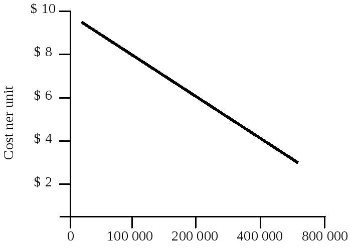
Figure 1-B. Cost per unit as a function of accumulated production the experience curve
If a downward-sloping experience curve exists, this is highly significant for the company. Not only will the company’s unit production cost fall, but it will fall faster if the company makes and sells more during a given time period. But the market has to stand ready to buy the higher output. And to take advantage of the experience curve, TI must get a large market share early in the product’s life cycle. This suggests the following pricing strategy. TI should price its calculators low; its sales will then increase, and its costs will decrease through gaining more experience, and then it can lower its prices further.