

Книги по МРТ КТ на английском языке / MRI for Orthopaedic Surgeons Khanna ed 2010
.pdf10 I Initial Concepts
Fig. 1.9 An axial T1-weighted conventional SE image through the left pelvis shows a lesion in the iliac fossa with areas of increased signal (arrow), which represent a hematoma in a patient with hemophilia. The di erential diagnosis for T1 hyperintense material includes fat, hemorrhage in the form of methemoglobin, gadolinium-based contrast material, proteinaceous material, some forms of calcium (when in solution), and melanin (as may be seen in melanoma).
to show intermediate signal intensity that is somewhere between that of collagenous tissue and fat. Usually, the higher the protein content of the fluid, the brighter the fluid appears on T1-weighted images. For the assessment of tumors or musculoskeletal infection, fat-suppressed T1-weighted imaging after gadolinium contrast administration represents the sequence of choice because the high signal from fat is suppressed, making enhancement of abnormal tissue more conspicuous (Fig. 1.11). Short scan times (because of the relatively short TRs) and excellent spatial resolution and depiction of anatomic detail are the major advantages of a T1-weighted pulse sequence. Its major weakness is the relative lower sensitivity for detecting soft-tissue edema compared with fluid-sensitive sequences such as fat-suppressed T2-weighted and STIR sequences.3
T2-weighted SE and T2-weighted FSE
T2-weighted SE and FSE sequences use a relatively long TE and long TR to maximize the T2 di erences in the tissues. Both sequences, when combined with fat suppression, are excellent for detecting edema/fluid, which appears bright and is often associated with pathologic processes such as tumors, infection, fractures, tenosynovitis, and bone contu-
sions (Fig. 1.12). The T2-weighted SE and FSE sequences also are good for evaluating ligaments and tendons, cartilage, and fluid-filled structures such as cysts. As on T1-weighted SE sequences, air, cortical bone, calcified structures, and fast-flowing blood appear dark on T2-weighted sequences. Hyperacute blood (oxyhemoglobin) and subacute blood (extracellular methemoglobin) are bright on T2-weighted SE and FSE sequences. These sequences also have been shown to be useful for di erentiating between fluid and tissue with a high fluid content, such as articular cartilage. The T2weighted sequences (especially the FSE sequences) may be used in evaluating for articular cartilage defects.
One of the limitations of standard T2-weighted SE sequences is the relatively long image acquisition times. FSE imaging represents a technical innovation that permits much more rapid imaging with T2 contrast7 with the use of multiple 180-degree RF pulses to create multiple echoes during a single TR period. The series of echoes is called the echo train, and the number of echoes produced in a single TR period is known as the echo train length. Because of their fast acquisition times, T2-weighted FSE sequences largely have replaced standard T2-weighted SE sequences.1,8
The major weakness of T2-weighted SE and T2-weighted FSE sequences is their inability to detect marrow pathology when not combined with fat-suppression techniques (Fig. 1.13). This limitation is secondary to the fact that both fat and water are bright on non–fat-suppressed T2-weighted FSE and SE sequences.3
Fig. 1.10 A sagittal T1-weighted SE image of the knee. Tendons and ligaments appear dark, fat is predominantly bright, and muscle has an intermediate signal.
1 Essentials of MRI Physics and Pulse Sequences |
11 |
A 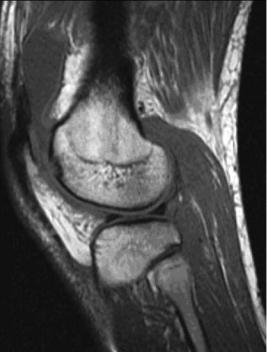 B
B
Fig. 1.11 Sagittal T1-weighted SE images after the intravenous administration of a gadolinium-based contrast material without (A) and with (B) fat suppression. The di use enhancement of the synovium
(arrow on B) is much more apparent with fat suppression in this patient with septic arthritis. The improved conspicuity is a major benefit of using fat suppression.
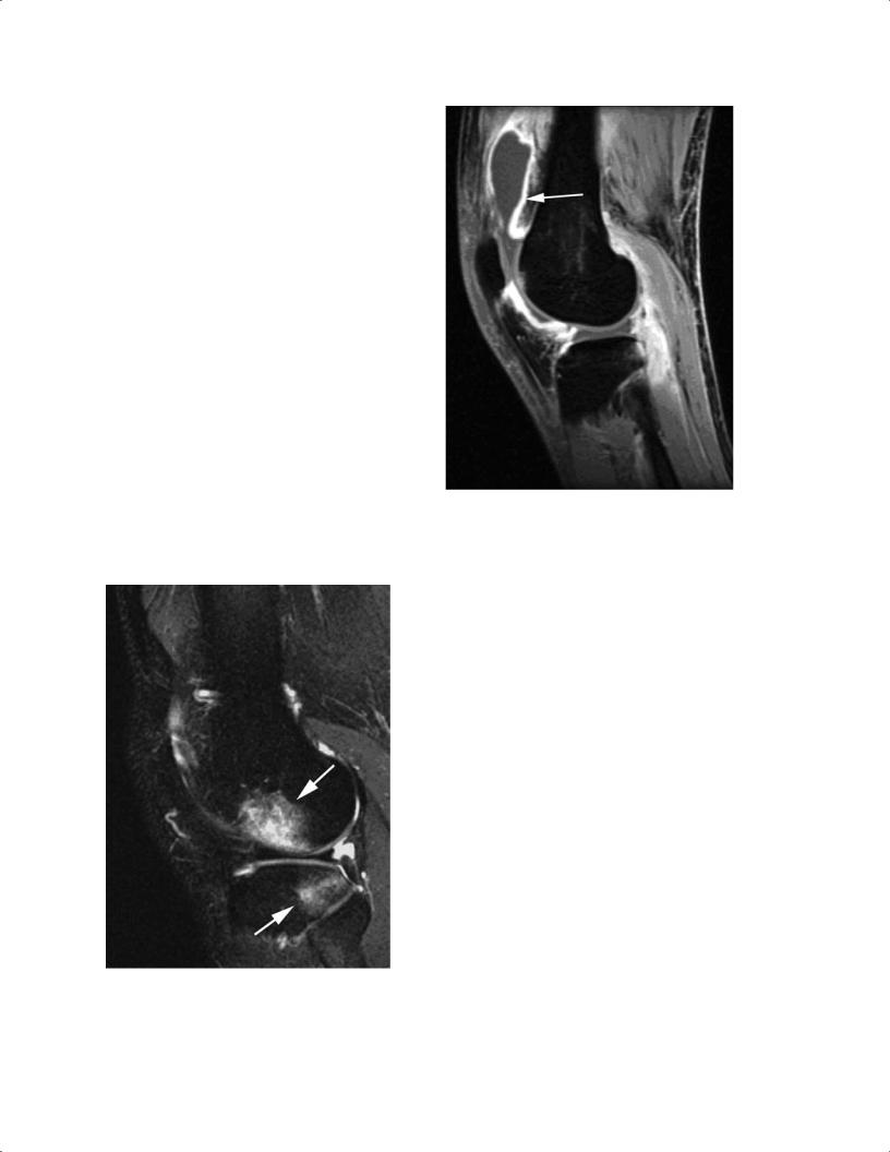
Fig. 1.12 A sagittal T2-weighted FSE image with fat suppression through the lateral compartment of the knee shows high signal within the distal femur and proximal tibia related to bone contusions
(arrows).
Proton-Density SE and Proton-Density FSE
Proton-density SE sequences and proton-density FSE sequences are excellent for depicting anatomic detail3 because of the high signal-to-noise ratio of proton-density–weighted images. Proton-density SE sequences also are used to evaluate regions obscured by high signal on T2-weighted images. Fat-suppressed proton-density imaging is often used for the MRI evaluation of meniscal and articular cartilage (Fig. 1.14).9
The major weakness of proton-density–weighted images is that tissue contrast is not as pronounced as with T1-weighted or T2-weighted images because proton-density– weighted images are a combination of T1 and T2 weighting.3 Therefore, proton-density–weighted SE sequences are not as sensitive for the detection of fluid and marrow pathology.3
Fat Suppression with T1-Weighted, T2-Weighted, and Proton-Density SE and FSE
Fat suppression commonly is achieved by spectral fat suppression or a STIR technique.10 Spectral fat-suppression imaging is restricted to MRI systems with midlevel and high magnetic field strength because of the necessity for identifying distinct fat and water resonance peaks and selectively suppressing the signal arising from adipose tissue, a process dependent on the presence of a relatively strong magnetic
12 I Initial Concepts
A 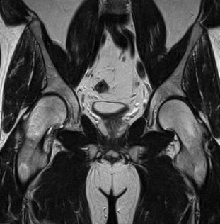
 B
B
Fig. 1.13 Coronal T2-weighted FSE images of the pelvis and hips without (A) and with (B) fat suppression. Increased signal within the right proximal femur related to transient osteoporosis (transient
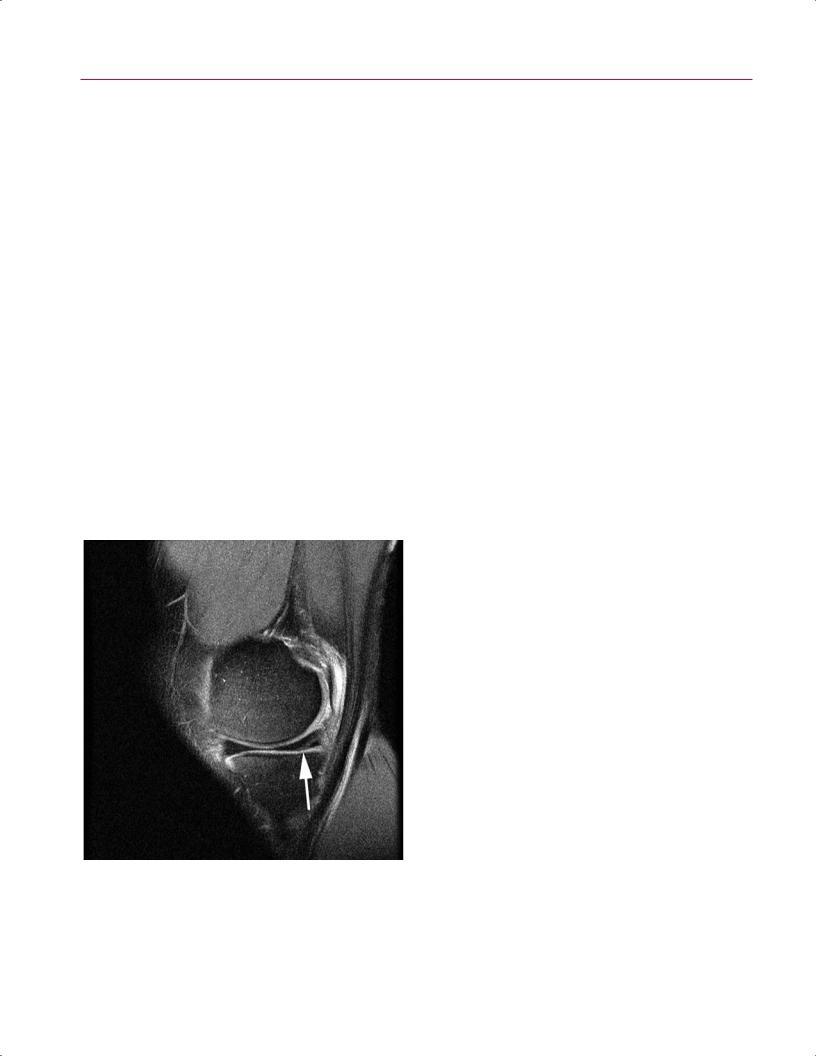
Fig. 1.14 A sagittal proton-density (intermediate)-weighted FSE image with fat suppression through the medial compartment of the knee, showing an arthroscopically proven meniscal tear. Linear signal is present in the posterior horn of the medial meniscus extending obliquely to the undersurface (arrow). This type of sequence is very useful for evaluating the internal derangement of joints.
bone marrow edema syndrome) is seen much more easily with fat suppression (arrow on B) and is inconspicuous on the FSE image that is not fat suppressed.
field. When combined with T2-weighted or proton-den- sity-weighted imaging, this technique is particularly useful in detecting bone bruises and osseous stress injury; the hyperintense intraosseous fluid that accumulates secondary to osseous contusion and microtrabecular fractures appears particularly conspicuous in contrast to the adjacent suppressed normal marrow fat signal.11
On T1-weighted images, fat suppression can allow for the di erentiation of fat-containing masses, for example, lipoma/ liposarcoma, from other tissue that may contain elements of increased signal (e.g., hemorrhage within tissue). Additionally, it can be used to verify the presence of fat within a lesion and to increase the conspicuity of enhancing masses on contrast-enhanced T1-weighted images.
One of the disadvantages of T2, T1, and proton-density fat-suppression sequences is incomplete suppression of the signal from fat secondary to local magnetic field inhomogeneities and susceptibility e ects (Fig. 1.15).3 This e ect is most prominent with images of curved surfaces, such as in the shoulder and ankle, or of any body part in the presence of metal or air. Additionally, as mentioned above, fat suppression requires higher strength magnets (>1 T) to ensure proper fat suppression than is generally required for non– fat-suppression MRI. STIR sequences often are used to overcome the e ects of magnetic field inhomogeneities seen with fat-suppression techniques (see the section below).
1 Essentials of MRI Physics and Pulse Sequences |
13 |
RF pulse after inversion time to nullify the signal from fat. Because of this phase-refocusing inversion pulse, STIR sequences are less susceptible to magnetic field inhomogeneities and subsequent susceptibility e ects that often result in inhomogeneous fat suppression on SE and FSE sequences. One of the major weaknesses of the STIR sequence, however, is that it suppresses the signal from all tissue with T1 signal characteristics similar to those of fat. Therefore, STIR pulse sequences should not be used with gadolinium contrast because gadolinium has relaxation properties similar to those of fat tissue, and thus all tissue with the same inversion time as fat (e.g., certain types of hemorrhage, melanin, and proteinaceous fluid) also will have its signal suppressed.3
Gradient Echo, 3D Gradient Echo
As indicated above, gradient-echo MRI pulse sequences use gradients to recall the echo at TE. Specifically, a negative gradient is followed by a positive gradient to refocus the signal at readout. As described above, in gradient-echo sequences, the TR varies and is related to the flip angle and the TE. A large flip angle (70 to 110 degrees) and a short TE favor T1 weighting, whereas a small flip angle (5 to 20 degrees) and a large TE favor T2* weighting. A low flip angle and a short TE result in a proton-density–weighted image.
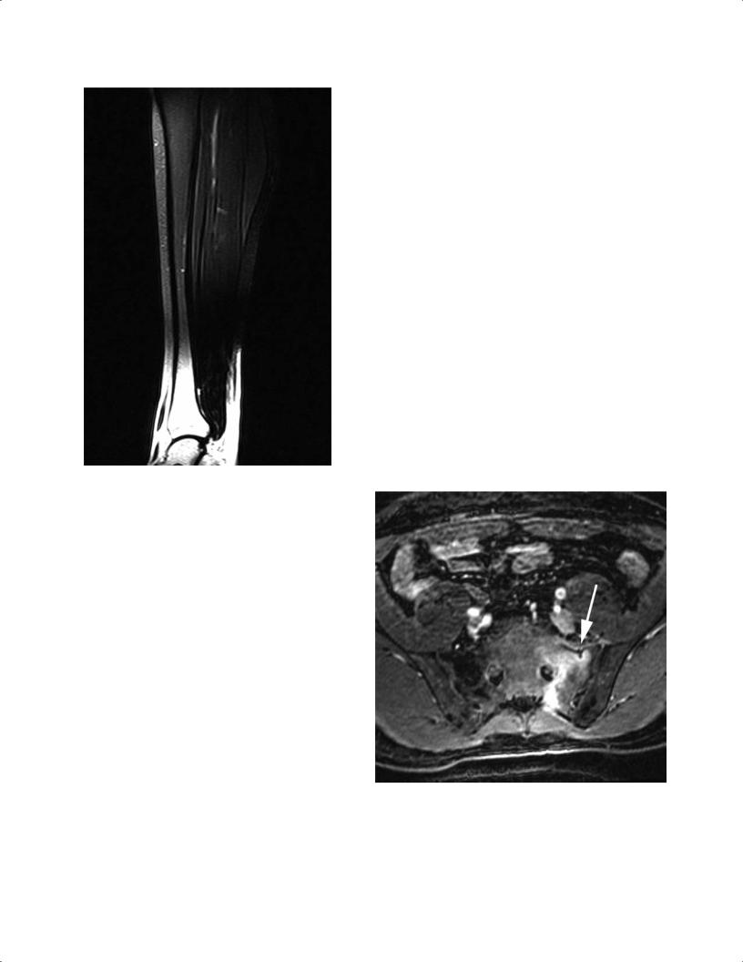
Fig. 1.15 A sagittal T1-weighted SE image of the leg shows suppression of the signal from fat; the distal leg shows bright signal in the marrow and subcutaneous regions. One of the weaknesses of chemically selective fat-suppression techniques is this incomplete fat suppression, which results from local field heterogeneity. This incomplete fat suppression may arise if the imaging is o isocenter (outside of the “sweet spot” of the magnet), such as in the wrist or elbow, when there are noncylindrical structures with materials of substantially di erent magnetic susceptibilities next to each other (soft tissue and air), such as the foot, or with large field of views.
STIR
STIR is another MRI pulse sequence commonly used in musculoskeletal imaging and, like T2-weighted sequences with fat suppression, is excellent for detecting fluid and edema when administered with a long TE. STIR can be used as an alternative to T2-weighted imaging. On fluid-sensitive-images such as STIR, fluid appears bright and makes the edema and fluid associated with certain types of pathology more conspicuous (Fig. 1.16) than they are on non–fluid-sensitive sequences. Such pathology includes osteomyelitis, fasciitis, abscesses, metastases, primary bone tumors, fractures, tenosynovitis, tendon tears, and bone contusions. Unlike T1weighted and T2-weighted fat-suppression sequences, STIR uses a 180-degree RF inversion pulse, followed by a 90-degree
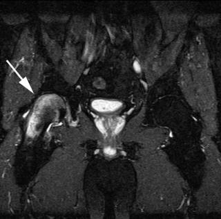
Fig. 1.16 An axial STIR image of the pelvis shows increased signal within the left side of the sacrum. A small incomplete fracture line is present within the anterior cortex (arrow). These findings represent an insu ciency-type stress fracture. Note that the signal from fat is very uniformly suppressed with the use of this pulse sequence.
14 I Initial Concepts
Gradient-echo sequences are more sensitive than SE sequences to local magnetic field inhomogeneities. These inhomogeneities can be created by blood, air, or calcium within tissue or can be intrinsic to the MRI unit itself. As a result, gradient-echo sequences are very sensitive for the detection of certain types of tissue, such as calcification, focal air collections, and blood products, that produce magnetic field inhomogeneity. Similarly, gradient-echo sequences of tissue that contains surgical instrumentation (metal) tend to produce substantial artifact secondary to the disturbance in the local magnetic field created by that instrumentation. Because of the susceptibility e ects of the trabecular bone, gradient-echo images also tend to overestimate the size or prominence of osteophytes within the spine and marrow pathology when the trabecular bone is not destroyed.3
Susceptibility artifacts seen on gradient-echo sequences can be helpful in identifying diseases such as PVNS because the hemosiderin deposits that are characteristic of the disease produce local magnetic field inhomogeneities that result in focal susceptibility artifacts.
Gradient-echo sequences also can be used to detect abnormalities involving the glenoid labrum and menisci of the knee; however, the contrast between other soft tissues (such as muscle and fat) is relatively poor compared with that of other pulse sequences. Gradient-echo sequences may be T2* weighted, T1 weighted, or proton-density weighted, depending on what tissue is being evaluated.
In 3D gradient-echo sequences, signal from an entire volume of tissue (i.e., in the x, y, and z planes) is acquired at the same time. This volume of tissue then may be partitioned into sections in any plane. These sections obtained from the 3D volume data set may be isotropic, or nearly so, and can be oriented in any way that is helpful for interpreting the data set. In general, 3D sequences (also known as volume acquisitions) have a higher signal-to-noise ratio because an entire volume of tissue is sampled rather than a single thin section. This optimal signal-to-noise ratio makes the 3D acquisition pulse sequences especially useful at low field strengths.4 Additionally, relatively high resolution and the high signal-to- noise ratio make the 3D gradient-echo sequences good for detecting abnormalities within small structures, such as the ligaments in the wrist3 and the articular cartilage.3,4,12 The major disadvantages of 3D gradient-echo pulse sequences are the relatively long acquisition times and the tendency toward susceptibility and motion artifacts.
Contrast-Enhanced Imaging
Gadolinium is commonly used as an intravenous and intraarticular contrast agent in musculoskeletal imaging. Its function in intravenous imaging is analogous to that of the iodinated contrast agent used in CT, and tissues that show increased vascularity generally show enhancement on postcontrast T1-weighted images. Fat-suppression techniques are
commonly used with gadolinium because of their sensitivity to detecting gadolinium.12 Areas in which there is breakdown of the blood–brain barrier also show enhancement. Specific uses for intravenous contrast include the evaluation of spinal lesions and di erentiation of the following3,12:
•Solid from cystic lesions
•Soft-tissue phlegmon from inflammation from abscess
•Surgical scars from disc fragments
Intravenous administration also can be used in indirect MR arthrography.
MR arthrography and the intraarticular administration of gadolinium involve the direct injection of a gadolinium contrast solution into the joint. MR arthrography has the advantage of being able to provide joint distention and is especially helpful in delineating labral tears in the hip and shoulder, ligamentous injuries, and TFCC tears in the wrist (Fig. 1.17). In the knee, MR arthrography has also been proposed as a technique that may improve sensitivity and specificity in detecting articular cartilage pathology, loose bodies, and meniscal tears, particularly in the postoperative knee.13,14 Disadvantages include the relatively invasive
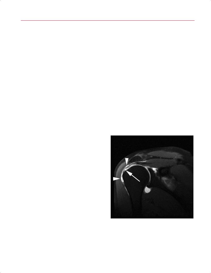
Fig. 1.17 This coronal T1-weighted SE image through the right shoulder with fat suppression after the intraarticular administration of a dilute gadolinium-based contrast material shows a full-thickness rotator cu tear as a defect involving the supraspinatus tendon (arrow). Note that the hyperintense contrast material extends from the fullthickness defect and is present within the subacromial/subdeltoid bursa (arrowheads).

|
|
1 Essentials of MRI Physics and Pulse Sequences 15 |
|||
nature of the procedure, the potential for introducing air |
tendons and cartilage when they are oriented at or near 55 |
|
|||
bubbles that could simulate loose bodies, and leakage of |
degrees to the main magnetic field. |
||||
paramagnetic contrast material into the periarticular tissues |
|
|
|
||
that could obscure or mimic pathology. |
|
|
|
||
Indirect arthrography involves the intravenous injection |
|
|
|
||
of gadolinium contrast material and imaging the joint ap- |
■ Summary |
||||
|
|
|
|||
proximately 5 to 10 minutes after injection, following move- |
|
|
|
||
ment of the joint through its range of motion. An alternative |
A fundamental knowledge base of MRI physics is important |
||||
technique images the joint immediately after injection, |
for the optimal use of MRI technology. This imaging modality |
||||
focusing on the enhancement of abnormal periarticular |
is well suited for evaluating musculoskeletal disease because |
||||
tissue or hyperemia rather than using the arthrographic |
it provides an accurate anatomic assessment, which is of par- |
||||
e ect provided by direct and indirect MR arthrography. |
amount importance. RF pulses, appropriately applied within |
||||
With this technique, contrast material rapidly di uses into |
a graded magnetic field, can localize the tissue of interest, |
||||
the synovial fluid, facilitated by joint movement, provid- |
and the signal produced can be Fourier-transformed into an |
||||
ing an arthrographic appearance without directly violating |
image. This image is defined not only by the T1, T2, and T2* |
||||
the joint.15,16 In patients with inflammatory arthritis, this |
relaxation time constants of the specific tissue, but also by |
||||
technique proves particularly useful in evaluating synovial |
the parameters that are used to assess the region of interest. |
||||
thickening. |
The primary pulse sequence parameters in MRI are TE, TR, |
||||
|
|
and inversion time, and these values determine the weight- |
|||
|
|
ing of the image (e.g., T1, T2, or proton-density), the strength |
|||
|
|
of the signal, and whether a certain type of tissue (e.g., fat) |
|||
■ Artifacts |
is suppressed. Each of the standard pulse sequences used in |
||||
musculoskeletal imaging (SE, FSE, STIR, and gradient echo) |
|||||
|
|
||||
Common artifacts seen in MRI include motion artifacts, |
has its own strengths and weaknesses, and a combination |
||||
truncation artifacts, the magic angle e ect, and susceptibil- |
of various sequences is typical for evaluation of the joints |
||||
ity e ects. |
and spine. T1-weighted images are optimal for showing ana- |
||||
Motion artifacts in MRI are common and are directly re- |
tomic detail, bone/bone marrow abnormalities, and carti- |
||||
lated to patient motion within the scanner. Patient motion |
lage tears, and they are excellent, when combined with fat |
||||
results in misregistration of the MR signal and subsequent |
suppression, for showing abnormal contrast enhancement. |
||||
blurring of the MR image. Motion from the pulsation of arter- |
Conversely, T1-weighted images are not optimal for show- |
||||
ies results in a particular type of motion artifact or pulsation |
ing soft-tissue edema. T2-weighted images are excellent for |
||||
artifact. This type of artifact produces partial reproductions |
detecting edema/fluid and processes associated with an in- |
||||
of the pulsating vessel in the phase-encoding direction. |
creased fluid content, such as trauma and tumors. They also |
||||
Truncation artifacts occur in MRI and are related to the |
may be useful for articular cartilage evaluation but are rela- |
||||
way the MR signal is processed during image creation and, |
tively insensitive to marrow fluid unless combined with a fat- |
||||
in particular, to the Fourier transformation method used to |
suppression technique. Proton-density images provide the |
||||
process the MR signal data.17 Truncation artifacts that can be |
highest signal-to-noise ratio and are excellent for showing |
||||
seen include ring artifacts, artificial edge widening at par- |
anatomic detail. The primary disadvantage of proton-density |
||||
allel high-contrast interfaces, interface edge enhancement, |
sequences is the lack of pure contrast compared with that |
||||
and distortion of adjacent tissues at parallel high contrast |
of T1-weighted and T2-weighted images. Gradient-echo |
||||
interfaces.17 |
sequences are useful for detecting fibrocartilage tears and |
||||
Susceptibility artifacts seen in MRI, briefly discussed |
for identifying tissue such as blood or metal that causes |
||||
above, are the result of local field inhomogeneities within |
magnetic inhomogeneity. 3D gradient-echo sequences can |
||||
the scan field, which create areas of focal signal loss. These |
be obtained in one sequence and examined in any plane as a |
||||
magnetic field inhomogeneities can be related to the magnet |
volume of tissue. The primary disadvantage of 3D gradient- |
||||
or to metal, air, calcium, or blood products within the tissues |
echo imaging is the long acquisition time; the same suscep- |
||||
being imaged.3,4 |
tibility to magnetic field inhomogeneity that may be useful |
||||
The magic angle e ect is the result of the prolongation of |
is also a disadvantage when it obscures the tissue of interest. |
||||
T2 within tissues with highly ordered structures that are at |
Fat suppression may be accomplished by frequency-specific |
||||
a 55-degree angle relative to the main magnetic field.12 This |
suppression or by inversion recovery techniques. Frequency- |
||||
e ect can simulate pathology by producing increased signal, |
specific suppression is useful but may be a ected by mag- |
||||
such as that seen within a normal supraspinatus tendon. To |
netic field heterogeneity. Inversion recovery fat suppression |
||||
avoid overtreating a normal patient or structure, care should |
is homogeneous but also suppresses tissue with the same |
||||
be taken when evaluating highly structured tissues such as |
inversion time as fat. Gadolinium is used as a contrast agent, |
||||

16 I Initial Concepts
most often with frequency-specific fat suppression (because inversion recovery techniques may suppress the signal from the gadolinium). Intravenous injections also may be used for indirect arthrography, although direct injection of gadolinium often may be necessary to achieve optimal joint distention and visualization of the appropriate anatomy.
It is often said that MRI is a compromise and that no gain in image quality is obtained without sacrificing some other
References
1.Bitar R, Leung G, Perng R, et al. MR pulse sequences: what every radiologist wants to know but is afraid to ask. Radiographics 2006;26:513–537
2.Huda W, Slone RM. Review of Radiologic Physics. 2nd ed. Philadelphia: Lippincott William & Wilkins; 2003
3.Kaplan PA, Helms CA, Dussault R, Anderson MW, Major NM. Basic principles of musculoskeletal MRI. In: Kaplan PA, et al., eds. Musculoskeletal MRI. Philadelphia: WB Saunders; 2001:1–21
4.Runge VM, Nitz WR, Schmeets SH, Faulkner WH Jr, Desai NK. The Physics of Clinical MR Taught Through Images. New York: Thieme; 2005
5.Lejay H, Holland BA. Technical advances in musculoskeletal imaging. In: Stoller DW, ed. Magnetic Resonance Imaging in Orthopaedics and Sports Medicine. 3rd ed. Baltimore: Lippincott Williams & Wilkins; 2007:1–28
6.Wehrli FW, Shaw D, Kneeland JB. Biomedical Magnetic Resonance Imaging: Principles, Methodology, and Applications. New York: VCH Publishers; 1988
7.Mirowitz SA. Fast scanning and fat-suppression MR imaging of musculoskeletal disorders. AJR Am J Roentgenol 1993;161:1147–1157
8.Escobedo EM, Hunter JC, Zink-Brody GC, Wilson AJ, Harrison SD, Fisher DJ. Usefulness of turbo spin-echo MR imaging in the evaluation of meniscal tears: comparison with a conventional spin-echo sequence. AJR Am J Roentgenol 1996;167:1223–1227
9.Potter HG, Linklater JM, Allen AA, Hannafin JA, Haas SB. Magnetic resonance imaging of articular cartilage in the knee. An evaluation with use of fast-spin-echo imaging. J Bone Joint Surg Am 1998;80:1276–1284
portion of the sequence or the examination. A clear understanding of the basic elements of MRI, along with how these elements interact, allows the imager to adjust the scanning techniques and image protocols to obtain the highest quality images possible. This optimization is important in all subspecialty imaging but is especially so in musculoskeletal imaging, where elucidating the anatomy is fundamental to analyzing the structure for the presence of pathology.
10.Delfaut EM, Beltran J, Johnson G, Rousseau J, Marchandise X, Cotten A. Fat suppression in MR imaging: techniques and pitfalls. Radiographics 1999;19:373–382
11.Kapelov SR, Teresi LM, Bradley WG, et al. Bone contusions of the knee: increased lesion detection with fast spin-echo MR imaging with spectroscopic fat saturation. Radiology 1993;189:901–904
12.Stoller DW. Magnetic Resonance Imaging in Orthopaedics and Sports Medicine. 3rd ed. Philadelphia: Lippincott Williams & Wilkins; 2007
13.Brossmann J, Preidler KW, Daenen B, et al. Imaging of osseous and cartilaginous intraarticular bodies in the knee: comparison of MR imaging and MR arthrography with CT and CT arthrography in cadavers. Radiology 1996;200:509–517
14.Magee T, Shapiro M, Rodriguez J, Williams D. MR arthrography of postoperative knee: for which patients is it useful? Radiology 2003;229:159–163
15.Drapé JL, Thelen P, Gay-Depassier P, Silbermann O, Benacerraf R. Intraarticular di usion of Gd-DOTA after intravenous injection in the knee: MR imaging evaluation. Radiology 1993;188:227–234
16.Winalski CS, Aliabadi P, Wright RJ, Shortkro S, Sledge CB, Weissman BN. Enhancement of joint fluid with intravenously administered gadopentetate dimeglumine: technique, rationale, and implications. Radiology 1993;187:179–185
17.Czervionke LF, Czervionke JM, Daniels DL, Haughton VM. Characteristic features of MR truncation artifacts. AJR Am J Roentgenol 1988;151:1219–1228

2 Normal MRI Anatomy of the
Musculoskeletal System
J. Dana Dunleavy, A. Jay Khanna, and John A. Carrino
To evaluate e ectively an MRI examination of a particular joint or region in the musculoskeletal system, it is essential to have at least a basic understanding of the normal MRI anatomy of that region. Many excellent texts and atlases have been written to serve this need for clinicians and radiologists.1,2 This chapter provides a brief overview of the most clinically important anatomy for each major region of the musculoskeletal system. The figures and line drawings in this chapter serve to highlight the structures with which the musculoskeletal medicine provider should be familiar before interpreting an imaging examination of the region. Reviewing the normal anatomy images pertinent to a specific anatomic region before reading the corresponding region-specific chapter will enhance the clinician’s understanding of the relevant pathologic conditions and facilitate recognition and di erentiation of the subtle regional anatomic alternations that represent various pathologic conditions.
■ Shoulder
Axial Images
Axial images are obtained from the superior aspect of the AC joint through the inferior glenoid margin. Axial plane images are best used for evaluating the glenoid labrum (anterior and posterior portions) (Fig. 2.1) and capsular structures as well as the long head of the biceps tendon in the bicipital groove.3 In addition, these images provide good visualization of the subscapularis muscle and tendon, the humeral head, and the glenoid (Fig. 2.2). On superior axial images, the normal oblique course of the supraspinatus muscle is displayed with intermediate signal intensity, and the supraspinatus tendon is low in signal intensity. In cross-section, the tendon of the long head of the biceps is seen as a low signal intensity structure within the bicipital groove. Glenoid articular cartilage follows the concave shape of the glenoid cavity and shows intermediate signal intensity on T1-weighted and T2-weighted images. Articular cartilage of the glenohumeral joint is best evaluated on gradient-echo or fat-suppressed T2-weighted sequences.4–6 The glenohumeral ligaments, best visualized on axial images, have low signal intensity on all pulse sequences. The superior glenohumeral ligament is identified at the level of the coracoid and the biceps tendon. The MGHL is highly variable and may
be identified as a thin band or a cord between the anterior labrum and subscapularis or may not be visualized at all without capsular distention. The anterior band of the IGHL is visualized more inferiorly between the anterior inferior labrum and the subscapularis tendon.
Coronal Oblique Images
Coronal oblique images are obtained in a plane that is parallel to the course of the supraspinatus tendon; they tend to show shoulder anatomy and pathology in a plane that is familiar to most. The osseous structures of the shoulder are easily recognized (Fig. 2.3A) as they would be seen on an AP shoulder radiograph. Similarly, the sagittal oblique images show the osseous structures as they would be seen from a lateral view (Fig. 2.3B). The coronal oblique images should include the subscapularis muscle anteriorly and the infraspinatus and teres minor muscles posteriorly. Coronal oblique images are best used to evaluate the supraspinatus muscle and tendon (Fig. 2.4), the subacromial and subdeltoid bursa, and the AC joint. The long head of the biceps tendon and biceps attachment, the infraspinatus muscle and tendon, the glenoid labrum (superior and inferior portions), and the glenohumeral joint space can also be visualized in the coronal oblique plane. Each coronal oblique image should be evaluated systematically from anterior to posterior. On anterior coronal oblique images, the subscapularis muscle and tendon can be identified as the tendon courses from its origin in the subscapularis fossa to its insertion on the lesser tuberosity. However, the subscapularis muscle and tendon can be seen more clearly on axial images (Fig. 2.2). The long head of the biceps tendon is best seen in its intraarticular location on coronal oblique images. On anterior and midcoronal oblique images, the supraspinatus muscle and tendon are seen in continuity (Fig. 2.5). The supraspinatus originates in the supraspinatus fossa of the scapula and inserts on the superior facet of the greater tuberosity of the humerus. On coronal oblique images, the anatomy of the AC joint is best displayed at the level of the supraspinatus tendon. The AC joint should be evaluated for the shape of the acromion (Fig. 2.4) and the various ligaments around the shoulder (Fig. 2.6). The superior and inferior portions of the glenoid labrum, as well as the axillary pouch, are also clearly shown on coronal oblique
17
18 I Initial Concepts
Long head of biceps tendon in bicipital groove
Humeral head |
Greater |
Lesser tuberosity |
cartilage |
tuberosity |
|
|
|
|
Humeral |
|
|
head |
|
|
Deltoid m. (lateral)
Deltoid m. |
|
(posterior) |
Posterior labrum |
|
A
Deltoid m.
Biceps brachii tendon (short head)
Anterior labrum
Serratus anterior m.
Glenoid surface
Subscapularis m.
Subscapularis a.
Subscapularis n.
Infraspinatus m. |
B |
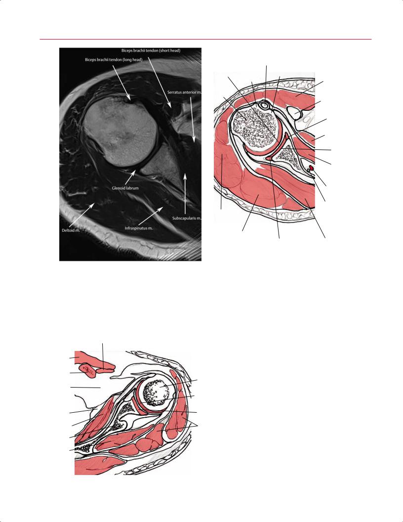
Fig. 2.1 An axial T2-weighted image (A) and artist’s sketch (B) of the right shoulder at the level of the glenoid labrum showing the long head of the biceps tendon as it courses along the bicipital groove.
|
Subclavius m. |
|
Pectoralis |
|
|
major m. |
|
|
Clavicle |
Head of |
|
|
||
|
humerus |
|
Axillary fat |
Humeral |
|
|
||
|
head |
|
|
cartilage |
|
Serratus |
Glenoid |
|
surface |
||
anterior m. |
||
|
||
Subscapularis m. |
Deltoid m. |
|
Scapular blade |
|
|
Infraspinatus m. |
|
Fig. 2.2 An axial illustration of the left shoulder showing the anterior position of the subscapularis muscle and the articular cartilage of the glenoid and humeral head.
|
|
2 |
Normal MRI Anatomy of the Musculoskeletal System |
19 |
||
|
AC joint |
Trapezoid lig. site |
Acromion |
Supraglenoid tubercle |
|
|
Acromion |
Clavicle |
|
||||
|
|
|
||||
|
Conoid lig. site |
|
|
|
|
|
|
|
|
|
|
|
|
Coracoid
Biceps tendon |
Biceps head, |
coracobrachialis |
|
origin, |
tendon site |
supraglenoid tubercle
|
Glenoid fossa |
Glenoid |
Surpascapular |
labrum |
notch and lig. |
Infraglenoid |
|
tubercle |
|
A |
|
B |
Fig. 2.3 Anterior (A) and lateral (B) 3D illustrations of the osseous structures of the right shoulder.
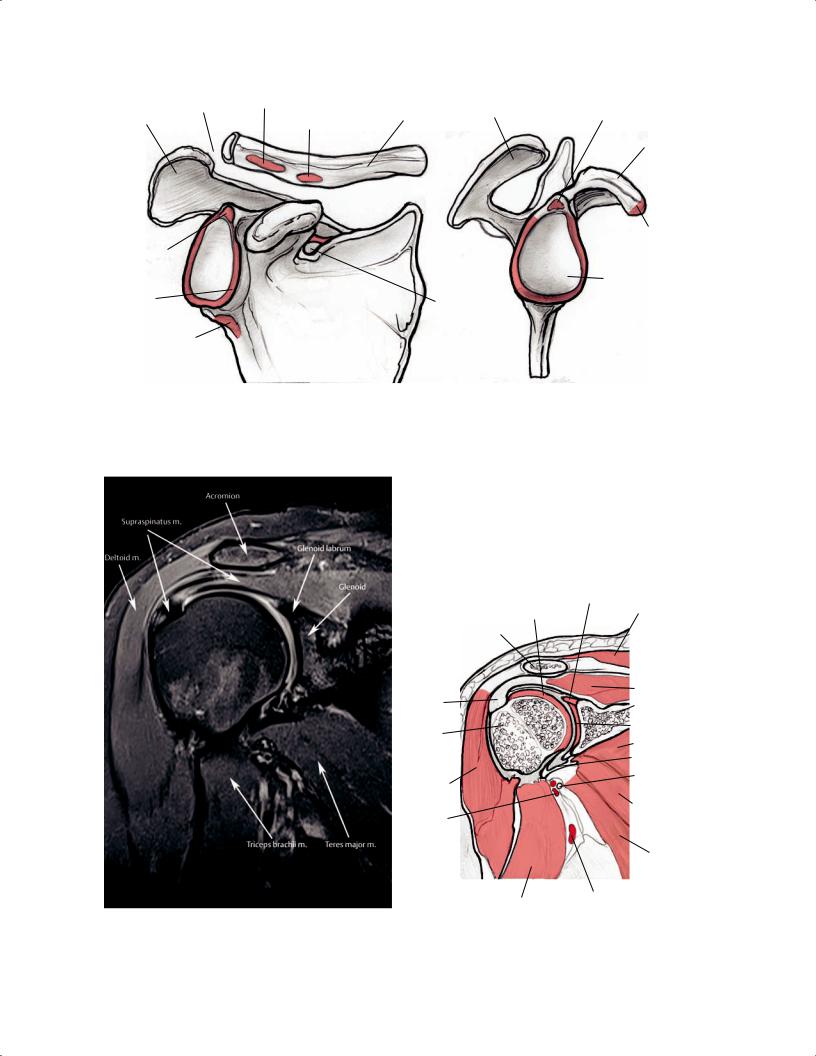
A
Fig. 2.4 A coronal proton-density fat-suppressed image (A) and artist’s sketch (B) of the right shoulder at the level of the supraspinatus muscle and the insertion of the conjoined tendon, a site that is very
|
Superior |
|
|
Humeral head |
glenoid labrum |
|
|
|
Trapezius m. |
||
cartilage |
|
||
Clavicle |
|
|
|
Conjoined |
|
Supraspinatus m. |
|
|
Scapula |
||
tendon |
|
||
|
|
Articular surface |
|
Humeral |
|
of glenoid |
|
|
|
|
|
head |
|
Subscapularis m. |
|
|
|
IGHL |
|
|
|
Axillary n. |
|
Deltoid m. |
|
|
|
Posterior |
|
Subscapularis m. |
|
|
|
|
|
circumflex |
|
|
|
humeral a. |
|
|
|
|
|
Teres major m. |
|
|
|
|
|
Triceps brachii m. |
Brachial a. |
|
B |
prone to rotator cu injury. The normal, flat acromion is also seen at this level, without evidence of supraspinatus impingement.