Chapter 12 HEAT TRANSFER ANALYSIS

The model at the beginning of this chapter is resumed from file: save_es-ice.4-final

The following tutorial data files are used in this chapter:

MAPPING_WALL_TEMPERATURE/cylinder_htx.dbs

MAPPING_WALL_TEMPERATURE/cylinder_htx.usr

MAPPING_WALL_TEMPERATURE/valves_htx.dbs

MAPPING_WALL_TEMPERATURE/valves_htx.usr

MAPPING_WALL_TEMPERATURE/engine.inp

The model at the end of this chapter is saved to file: save_es-ice.heat_transfer

es-ice can specify a non-uniform temperature boundary condition on a wall region instead of a Fixed or Adiabatic condition. The non-uniform wall temperature data can be obtained from any source, e.g. from a structural analysis or CFD code, or from experimental data.

In addition, you have the option of outputting calculated wall heat transfer data, e.g. wall heat fluxes, near-wall gas temperatures and wall heat transfer coefficients to a file called es-ice_htx.pos. Within es-ice, you can also cycle-average the wall heat transfer data and use them as boundary conditions for a structural analysis or post-processing run.

The steps for mapping non-uniform wall temperatures and post-processing heat transfer data are outlined below:

1.Map wall temperatures in es-ice

2.Export heat transfer data from the STAR solver

3.Cycle-average the heat transfer data obtained from the STAR solver

4.Post-process the heat transfer data in pro-STAR

5.Map the heat transfer data to an Abaqus model via STAR-CCM+

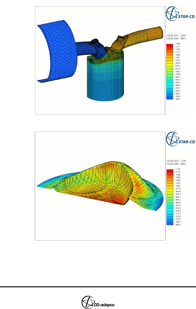
Figure 12-1, Table 12-2 and Table 12-3 show wall temperature data mapped as boundary conditions for various engine components.

Figure 12-1 Cylinder and port wall temperature boundary conditions

Figure 12-2 Piston wall temperature boundary conditions

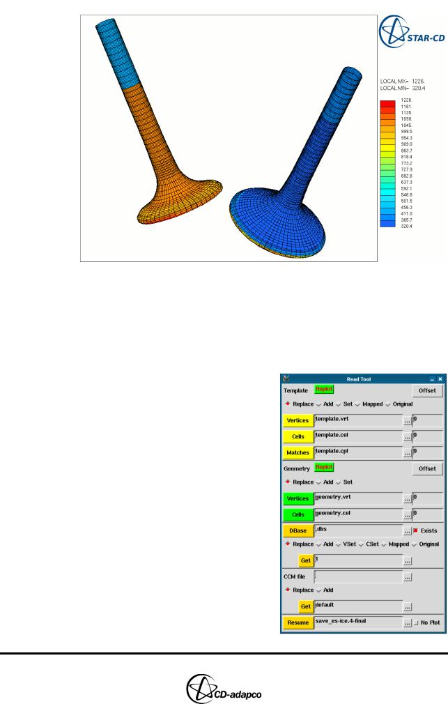
Figure 12-3 Valve wall temperature boundary conditions

Resuming the es-ice Model File

This tutorial starts from an es-ice model file created at the end of Chapter 6. The file contains data for a case study that is ready to be completed in pro-STAR and then run by the STAR solver. However, some of the boundary conditions and post-processing options need to be changed, as required for a heat transfer analysis.

To resume the es-ice model file:

•Ensure that save_es-ice.4-final is in your current working directory and launch es-ice in the usual manner

•In the Select panel, click Read Data

•In the Read Tool, click the ellipsis (...) next to the Resume box and select save_es-ice.4-final from the file browser

Mapping Wall Temperature

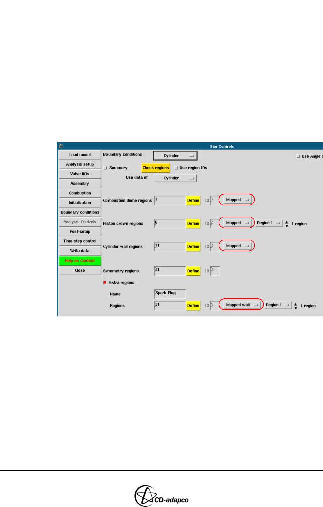
First, specify that the cylinder boundary regions are to use mapped wall temperature data.

•In the Select panel, click Star Controls

•In the Star Controls panel, open the Boundary conditions view

•Select the Cylinder domain from the drop-down menu at the top of the panel

•Set boundary conditions for the following boundary regions, as shown in Figure 12-4:

•Combustion dome regions: Mapped

•Piston crown regions: Mapped

•Cylinder wall regions: Mapped

•Extra regions > Spark Plug: Mapped Wall

[

Figure 12-4 Star controls panel: Boundary conditions view for the Cylinder

Similarly, specify that the intake port and valve regions are to use mapped wall temperature data.

•Select the Port and Valve 1 domain from the drop-down menu at the top of the panel

•As before, set boundary conditions for the following boundary regions, as shown in Figure 12-5:

•Valve stem regions: Mapped

•Valve face regions: Mapped

•Port wall regions: Mapped

Figure 12-5 Star controls panel: Boundary conditions view for Port and Valve 1

•Set the same boundary conditions for Port and Valve 2, as shown in Figure 12-6

Figure 12-6 Star controls panel: Boundary conditions view for Port and Valve 2

In the following steps, specify the files required to map wall temperature data. The valves are mapped separately to avoid confusion when mapping temperatures in the valve seat region.

•Select the Global settings domain from the drop-down menu at the top of the panel, as shown in Figure 12-7

•Under Wall temperature mapping, set Dbase file to cylinder_htx.dbs and

Dbase ID to 1 to select the cylinder and port surfaces

•Set Temperature to cylinder_htx.usr to specify the wall temperature data file

•Check that the Map valves separately toggle button is selected so that you can specify separate files for the valves

•Under Map valves separately, set Dbase file to valves_htx.dbs and Dbase ID