APPENDIX

B

IPYTHON NOTEBOOKS

IPython notebooks are useful for logging your work. Here we suggest that you use them for logging and turning in homework assignments. You may also find them useful in other contexts such as laboratory work. The IPython Notebook interface is similar to Mathematica or Maple.

B.1 An interactive interface

An IPython notebook is a web-based environment for interactive computing. You can work in this environment interactively just as you would using the IPython shell (the interactive Python pane shown in the Canopy window figure). In addition, you can also store and run programs in an IPython notebook just like you would from the Code Editor window (see Canopy window). Thus, it would seem that an IPython notebook and the Canopy environments do essentially the same thing. Up to a point, that is true. In the final analysis, however, Canopy (or Spyder or some similar Python development environment) is generally more useful for developing, storing, and running code. An IPython Notebook, on the other hand, is excellent for logging your work in Python. That is why we suggest using them for homework assignments. You may well find them useful in other contexts as well.

B.2 Installing and launching an IPython notebook

If you have installed Canopy, then you have already installed all the software you need to use IPython notebooks. IPython notbooks are stored in files with a .ipynb extension. To create an IPython notebook, launch the Terminal (Mac) or the Command Prompt (PC)

183

Introduction to Python for Science, Release 0.9.23

application. On the Mac, the Terminal application is found in the Applications/Utilies folder. On the PC, the Command Prompt application is found under the Start/All Programs/Accessories menu. Here we will refer the the Terminal or Command Prompt applications at the System Console. Type pwd (Mac) or chdir (PC) to determine the current directory (folder) of the System Console. Type ls (Mac) or dir (PC) to list all the files and subdirectories in the current directory. Using the cd change directory command, move the System Console to the directory in which you want to store your IPython notebook.

At the System Console prompt, type

ipython notebook --pylab inline

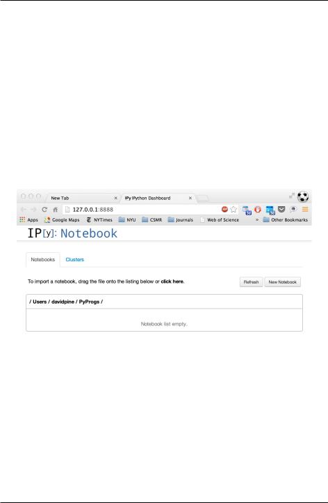
This will launch the IPython notebook web application and will display the IPython Notebook Dashboard as a page in your default web browser.

Figure B.1: IPython Notebook Dashboard

To create a new IPython notebook, click the New Notebook button. That will open a new IPython Notebook with the provisional title Untitled0 in a new tab in your browser. To give the notebook a more meaningful name, click on the File menu and select Rename.... Let’s say you rename your notebook FirstNotebook. The Name FirstNotebook will replace Untitled0 in your Notebook browser window and a file named FirstNotebook.ipynb will appear in the directory from which you launched IPython Notebook. That file will contain all the work you do in the IPython notebook. Next time you launch IPython Notebook from this same directory, all the

Introduction to Python for Science, Release 0.9.23

IPython notebooks in that directory will appear in a list on the IPython Notebook Dashboard. Clicking on one of them will launch that notebook.

Figure B.2: IPython Notebook

B.3 Using an IPython Notebook

When you open a new IPython Notebook, an IPython interactive cell with the prompt In[ ]: to the left, appears. You can type code into this cell just as you would in the IPython shell of the Canopy window. For example, typing 2+3 into the cell and pressing Shift-Enter (or Shift-Return) to execute the cell yields the expected result. Try it out.

Below the result a new IPython interactive cell appears ready for your next entry. Because we launched IPython Notebook with the --pylab switch, NumPy and MatPlotLib are already loaded so we do not need the np. or plt. prefixes to access the functions in the NumPy and MatPlotLib libraries. Thus, typing sin(pi/6.) and pressing Shift-Enter produces the expected result (to nearly 1 part in 1016).

You can also create plots in an IPython notebook. For example, typing plot([1,2,3,2,3,4,3,4,5]) and pressing Shift-Enter produces the same plot shown in Interactive plot window. The plot is produced “in line” and not in a separate window, because we used the inline switch when we launched IPython Notebook. If you have followed along, your IPython notebook should look something like that shown in the figure IPython Notebook demo.

Be sure to press the Save and Checkpoint icon at the far left near the top of the IPython Notebook window from time to time to save your work.

Introduction to Python for Science, Release 0.9.23

Figure B.3: IPython Notebook demo

Introduction to Python for Science, Release 0.9.23

B.4 Running programs in an IPython Notebook

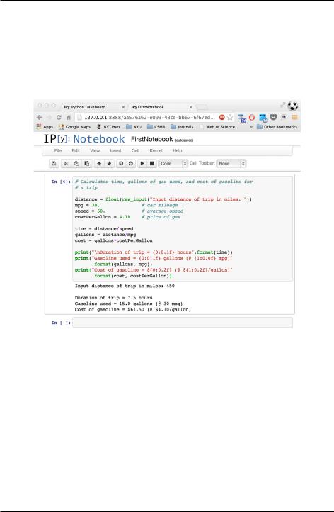
You can also run programs in an IPython notebook. As an example, we run the program introduced in the section on Screen output. The program is input into a single notebook cell and then executed by pressing Shift-Enter.

Figure B.4: Running a program

In this example, the program requests input from the user: the distance of the trip. The program runs up to the point where it needs input from the user, and then pauses until the user responds and presses the Enter or Return key. The program then completes its execution. Thus the IPython notebook provides a complete log of the session.

B.5 Annotating an IPython Notebook

An IPython notebook will be more easily comprehended if it includes annotations of the session. In addition to logging the inputs and outputs of computations, IPython Notebook

Introduction to Python for Science, Release 0.9.23

allows the user to embed headings, explanatory notes, mathematics, and images.

Figure B.5: Annotating a notebook

Suppose, for example, that we want to have a title at the top of the IPython notebook we have been working with, and we want to include the name of the author of the session. To do this, we scroll the IPython notebook back up to the top and place the cursor and click in the very first input cell, the one that contained 2+3. We then open the Insert menu near the top center of the window and click on Insert Cell Above, which opens up a new input cell above the first cell. Next, we click on the box in the Toolbar that says Code. A list of cell types appears: Code (currently checked), Markdown,

Raw Text, Heading 1, Heading 2, ..., Heading 6. Select Heading 1; immediately the In [ ]: prompt disappears, indicating that this box is no longer meant for inputing and executing Python code. Type “Demo of IPython Notebook” and press Shift-Enter (or Shift-Return). A heading in large print appears before the first IPython code cell. Place the cursor back in the first Ipython code cell (2+3). Once again, select the Insert menu and click on Insert Cell Above. Again, click on the Toolbar that says Code, but this time select Heading 2. Type your name into the newly created cell and press Shift-Enter. Your name is printed in the cell in slightly smaller print than for the previous case.

You can also write comments, including mathematical expressions, into an IPython Notebook cell. Let’s include a comment after the program we ran that calculated the cost of gasoline for a road trip. First we place the cursor in the open formula cell below program we ran and then click on the box in the Toolbar that says Code and change it to Markdown. Returning to the cell, we enter the text of our

Introduction to Python for Science, Release 0.9.23

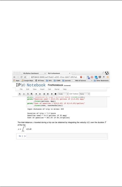
comment. We can enter any text we wish, including mathematical expressions using the markup language Latex. (If you do not already know Latex, you can get a brief introduction at these sites: http://en.wikibooks.org/wiki/LaTeX/Mathematics or ftp://ftp.ams.org/pub/tex/doc/amsmath/short-math-guide.pdf.) Here we enter the following text:

The total distance $x$ traveled during a trip can be obtained by integrating the velocity $v(t)$ over the duration $T$ of the trip:

\begin{align}

x = \int_0^T v(t)\, dt \end{align}

After entering the text, pressing Shift-Enter yields the result shown in Annotation using a Markdown cell.

Figure B.6: Annotation using a Markdown cell

The $ symbol brackets inline mathematical expressions in Latex, while the \begin{align} and \end{align} expressions bracket displayed expressions. You only need to use Latex if you want to have fancy mathematical expressions in your notes. Otherwise, they are not necessary.

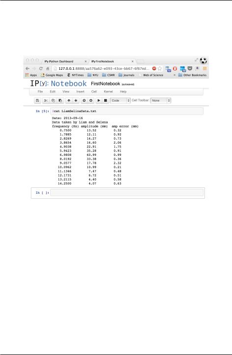
Suppose you were importing a data (.txt) file from your hard disk and you wanted to print it out in one of the notebook cells. If you were in the Terminal (Mac) or Command

Introduction to Python for Science, Release 0.9.23

Prompt (PC), you could write the contents of any text file using the command cat filename (Mac) or type filename (PC). You can execute the same operation from the IPython prompt using the Unix (Mac) or DOS (PC) command preceded by an exclamation point, as described in the section on System shell commands.

Figure B.7: Displaying a text file from disk

B.6 Editing and rerunning a notebook

In working with an IPython notebook, you may find that you want to move some cells around, or delete some cells, or simply change some cells. All of these tasks are possible. You can cut and paste cells, as in a normal document editor, using the Edit menu. You can also freely edit cells and re-execute them by pressing Shift-Enter. Sometimes you may find that you would like to re-execute the entire notebook afresh. You can do this by going to the Kernel menu and selecting Restart. A warning message will appear asking you if you really want to restart. Answer in the affirmative. Then open the Cell menu and select Run All, which will re-execute the notebook starting with the first cell. You will have to re-enter any screen input requested by the notebook scripts.

Introduction to Python for Science, Release 0.9.23

B.7 Quitting an IPython notebook

It goes almost without saying that before quitting an IPython notebook, you should make sure you have saved the notebook by pressing the Save and Checkpoint item in the File menu or its icon in the Toolbar.

When you are ready to quit working with a notebook, click on the Close and halt item in the File menu. Your notebook browser tab will close and you will return to the IPython Notebook Dashboard. Just close the IPython Notebook Dashboard tab in your browser to end the session.

Finally, return to the Terminal or Command Prompt application, hold down the control key and press c twice in rapid succession. This stops the IPython Notebook session. You should see the normal system prompt. You can then close the Terminal (Mac) or Command Prompt (PC) session if you wish.

B.8 Working with an existing IPython notebook

To work with an existing IPython notebook, open the Terminal (Mac) or Command Prompt (PC) application and navigate to the directory in which the notebook you want to work with resides. Recall that IPython notebooks have the .ipynb extension. Launch the IPython Notebook Dashboard as you did previously by issuing the command

ipython notebook --pylab inline

This will open the IPython Notebook Dashboard in your web browser, where you should see a list of all the IPython notebooks in that directory (folder). Click on the name of the notebook you want to open. It will appear in a new tab on your web browser as before.

Note that while all the input and output from the previous saved session is present, none of it has been run. That means that none of the variables or other objects has been defined in this new session. To initialize all the objects in the file, you must rerun the file. To rerun the file, press the Cell menu and select Run All, which will re-execute all the cells. You will have to re-enter any screen input requested by the notebook scripts. Now you are ready to pick up where you left off the last time.

Introduction to Python for Science, Release 0.9.23