CHAPTER

SEVEN

FUNCTIONS

As you develop more complex computer code, it becomes increasingly important to organize your code into modular blocks. One important means for doing so is user-defined Python functions. User-defined functions are a lot like built-in functions that we have encountered in core Python as well as in NumPy and Matplotlib. The main difference is that user-defined functions are written by you. The idea is to define functions to simplify your code and to allow you to reuse the same code in different contexts.

The number of ways that functions are used in programming is so varied that we cannot possibly enumerate all the possibilities. As our use of Python functions in scientific program is somewhat specialized, we introduce only a few of the possible uses of Python functions, ones that are the most common in scientific programming.

7.1 User-defined functions

The NumPy package contains a plethora of mathematical functions. You can find a listing of the mathematical functions available through NumPy on the web page http://docs.scipy.org/doc/numpy/reference/routines.math.html. While the list may seem pretty exhaustive, you may nevertheless find that you need a function that is not available in the NumPy Python library. In those cases, you will want to write your own function.

In studies of optics and signal processing one often runs into the sinc function, which is defined as

sinc x sinxx :

Let’s write a Python function for the sinc function. Here is our first attempt:

115

Introduction to Python for Science, Release 0.9.23

def sinc(x):

y = np.sin(x)/x return y

Every function definition begins with the word def followed by the name you want to give to the function, sinc in this case, then a list of arguments enclosed in parentheses, and finally terminated with a colon. In this case there is only one argument, x, but in general there can be as many arguments as you want, including no arguments at all. For the moment, we will consider just the case of a single argument.

The indented block of code following the first line defines what the function does. In this case, the first line calculates sinc x = sin x=x and sets it equal to y. The return statement of the last line tells Python to return the value of y to the user.

We can try it out in the IPython shell. First we type in the function definition.

In [1]: def sinc(x):

...: y = sin(x)/x

...: return y

Because we are doing this from the IPython shell, we don’t need to import NumPy; it’s preloaded. Now the function sinc x is available to be used from the IPython shell

Inputs and outputs 4 and 5 verify that the function does indeed give the same result as an explicit calculation of sin x=x.

You may have noticed that there is a problem with our definition of sinc x when x=0.0. Let’s try it out and see what happens

In [6]: sinc(0.0)

Out[6]: nan

IPython returns nan or “not a number”, which occurs when Python attempts a division by zero, which is not defined. This is not the desired response as sinc x is, in fact, perfectly well defined for x = 0. You can verify this using L’Hopital’s rule, which you may have

Introduction to Python for Science, Release 0.9.23

learned in your study of calculus, or you can ascertain the correct answer by calculating the Taylor series for sinc x. Here is what we get

From the Taylor series, it is clear that sinc x is well-defined at and near x = 0 and that, in fact, sinc(0) = 1. Let’s modify our function so that it gives the correct value for x=0.

Now our function gives the correct value for x=0 as well as for values different from zero.

7.1.1 Looping over arrays in user-defined functions

The code for sinc x works just fine when the argument is a single number or a variable that represents a single number. However, if the argument is a NumPy array, we run into a problem, as illustrated below.

In [10]: x = arange(0, 5., 0.5)

In [12]: sinc(x)

----------------------------------------------------------

Introduction to Python for Science, Release 0.9.23

4else:

5y = np.sin(x)/x

ValueError: The truth value of an array with more than one element is ambiguous.

The if statement in Python is set up to evaluate the truth value of a single variable, not of multielement arrays. When Python is asked to evaluate the truth value for a multi-element array, it doesn’t know what to do and therefore returns an error.

An obvious way to handle this problem is to write the code so that it processes the array one element at a time, which you could do using a for loop, as illustrated below.

1def sinc(x):

3for xx in x: # loops over all elements in x array

4if xx==0.0: # adds result of 1.0 to y list if

6else: # adds result of sin(xx)/xx to y list if

8return np.array(y) # converts y to array and returns array

9

10import numpy as np

11import matplotlib.pyplot as plt

12

13x = np.linspace(-10, 10, 256)

14y = sinc(x)

15

16plt.plot(x, y)

17plt.axhline(color="gray", zorder=-1)

18plt.axvline(color="gray", zorder=-1)

19plt.show()

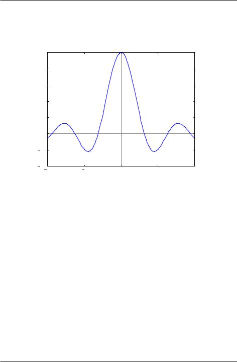
The for loop evaluates the elements of the x array one by one and appends the results to the list y one by one. When it is finished, it converts the list to an array and returns the array. The code following the function definition plots sinc x as a function of x.

In the program above, you may have noticed that the NumPy library is imported after the sinc(x) function definition. As the function uses the NumPy functions sin and array, you may wonder how this program can work. Doesn’t the import numpy statement have to be called before any NumPy functions are used? The answer it an emphatic “YES”. What you need to understand is that the function definition is not executed when it is defined, nor can it be as it has no input x data to process. That part of the code is just a definition. The first time the code for the sinc(x) function is actually executed is when it is called on line 14 of the program, which occurs after the NumPy library is

Introduction to Python for Science, Release 0.9.23

imported in line 10. The figure below shows the plot of the sinc x function generated by the above code.

Figure 7.1: Plot of user-defined sinc(x) function.

7.1.2 Fast array processing in user-defined functions

While using loops to process arrays works just fine, it is usually not the best way to accomplish the task in Python. The reason is that loops in Python are executed rather slowly. To deal with this problem, the developers of NumPy introduced a number of functions designed to process arrays quickly and efficiently. For the present case, what we need is a conditional statement or function that can process arrays directly. The function we want is called where and it is a part of the NumPy library. There where function has the form

where(condition, output if True, output if False)

The first argument of the where function is a conditional statement involving an array. The where function applies the condition to the array element by element, and returns the second argument for those array elements for which the condition is True, and returns the third argument for those array elements that are False. We can apply it to the sinc(x) function as follows

Introduction to Python for Science, Release 0.9.23

def sinc(x):

z = np.where(x==0.0, 1.0, np.sin(x)/x) return z

The where function creates the array y and sets the elements of y equal to 1.0 where the corresponding elements of x are zero, and otherwise sets the corresponding elements to sin(x)/x. This code executes much faster, 25 to 100 times, depending on the size of the array, than the code using a for loop. Moreover, the new code is much simpler to write and read. An additional benefit of the where function is that it can handle single variables and arrays equally well. The code we wrote for the sinc function with the for loop cannot handle single variables. Of course we could rewrite the code so that it did, but the code becomes even more clunky. It’s better just to use NumPy’s where function.

The moral of the story

The moral of the story is that you should avoid using for and while loops to process arrays in Python programs whenever an array-processing method is available. As a beginning Python programmer, you may not always see how to avoid loops, and indeed, avoiding them is not always possible, but you should look for ways to avoid loops, especially loops that iterate a large number of times. As you become more experienced, you will find that using array-processing methods in Python becomes more natural. Using them can greatly speed up the execution of your code, especially when working with large arrays.

7.1.3 Functions with more (or less) than one input or output

Python functions can have any number of input arguments and can return any number of variables. For example, suppose you want a function that outputs n (x; y) coordinates around a circle of radius r centered at the point (x0; y0). The inputs to the function would be r, x0, y0, and n. The outputs would be the n (x; y) coordinates. The following code implements this function.

def circle(r, x0, y0, n):

theta = np.linspace(0., 2.*np.pi, n, endpoint=False) x = r * np.cos(theta)

y = r * np.sin(theta) return x0+x, y0+y

This function has four inputs and two outputs. In this case, the four inputs are simple numeric variables and the two outputs are NumPy arrays. In general, the inputs and

Introduction to Python for Science, Release 0.9.23

outputs can be any combination of data types: arrays, lists, strings, etc. Of course, the body of the function must be written to be consistent with the prescribed data types.

Functions can also return nothing to the calling program but just perform some task. For example, here is a program that clears the terminal screen

import subprocess import platform

def clear():

subprocess.Popen( "cls" if platform.system() == "Windows" else "clear", shell=True)

The function is invoked by typing clear(). It has no inputs and no outputs but it performs a useful task. This function uses two standard Python libraries, subprocess and platform that are useful for performing computer system tasks. It’s not important that you know anything about them at this point. We simply use them here to demonstrate a useful cross-platform function that has no inputs and returns no values.

7.1.4 Positional and keyword arguments

It is often useful to have function arguments that have some default setting. This happens when you want an input to a function to have some standard value or setting most of the time, but you would like to reserve the possibility of giving it some value other than the default value.

For example, in the program circle from the previous section, we might decide that under most circumstances, we want n=12 points around the circle, like the points on a clock face, and we want the circle to be centered at the origin. In this case, we would rewrite the code to read

def circle(r, x0=0.0, y0=0.0, n=12):

theta = np.linspace(0., 2.*np.pi, n, endpoint=False) x = r * np.cos(theta)

y = r * np.sin(theta) return x0+x, y0+y

The default values of the arguments x0, y0, and n are specified in the argument of the function definition in the def line. Arguments whose default values are specified in this manner are called keyword arguments, and they can be omitted from the function call if the user is content using those values. For example, writing circle(4) is now a perfectly legal way to call the circle function and it would produce 12 (x; y) coordinates centered about the origin (x; y) = (0; 0). On the other hand, if you want the values of x0,

Introduction to Python for Science, Release 0.9.23

y0, and n to be something different from the default values, you can specify their values as you would have before.

If you want to change only some of the keyword arguments, you can do so by using the keywords in the function call. For example, suppose you are content with have the circle centered on (x; y) = (0; 0) but you want only 6 points around the circle rather than 12. Then you would call the circle function as follows:

circle(2, n=6)

The unspecified keyword arguments keep their default values of zero but the number of points n around the circle is now 6 instead of the default value of 12.

The normal arguments without keywords are called positional arguments; they have to appear before any keyword arguments and, when the function is called, must be supplied values in the same order as specified in the function definition. The keyword arguments, if supplied, can be supplied in any order providing they are supplied with their keywords. If supplied without their keywords, they too must be supplied in the order they appear in the function definition. The following function calls to circle both give the same output.

By now you probably have noticed that we used the keyword argument endpoint in calling linspace in our definition of the circle function. The default value of endpoint is True, meaning that linspace includes the endpoint specified in the second argument of linspace. We set it equal to False so that the last point was not included. Do you see why?

7.1.5 Variable number of arguments

While it may seem odd, it is sometimes useful to leave the number of arguments unspecified. A simple example is a function that computes the product of an arbitrary number of numbers:

def product(*args):

print("args = {}".format(args))

Introduction to Python for Science, Release 0.9.23

p = 1

for num in args: p *= num

return p

In [15]: product(11., -2, 3) args = (11.0, -2, 3) Out[15]: -66.0

In [16]: product(2.31, 7) args = (2.31, 7)

Out[16]: 16.17

The print("args...) statement in the function definition is not necessary, of course, but is put in to show that the argument args is a tuple inside the function. Here it used because one does not know ahead of time how many numbers are to be multiplied together.

The *args argument is also quite useful in another context: when passing the name of a function as an argument in another function. In many cases, the function name that is passed may have a number of parameters that must also be passed but aren’t known ahead of time. If this all sounds a bit confusing—functions calling other functions—a concrete example will help you understand.

Suppose we have the following function that numerically computes the value of the derivative of an arbitrary function f(x):

def deriv(f, x, h=1.e-9, *params):

return (f(x+h, *params)-f(x-h, *params))/(2.*h)

The argument *params is an optional positional argument. We begin by demonstrating the use of the function deriv without using the optional *params argument. Suppose we want to compute the derivative of the function f0(x) = 4x5. First, we define the function

def f0(x):

return 3.*x**5

Now let’s find the derivative of f0(x) = 4x5 at x = 3 using the function deriv:

In [17]: deriv(f0, 3)

Out[17]: 1620.0001482502557

The exact result is 1620, so our function to numerically calculate the derivative works pretty well.

Introduction to Python for Science, Release 0.9.23

Suppose we had defined a more general function f1(x) = axp as follows:

def f1(x, a, p): return a*x**p

Suppose we want to calculate the derivative of this function for a particular set of parameters a and p. Now we face a problem, because it might seem that there is no way to pass the parameters a and p to the deriv function. Moreover, this is a generic problem for functions such as deriv that use a function as an input, because different functions you want to use as inputs generally come with different parameters. Therefore, we would like to write our program deriv so that it works, irrespective of how many parameters are needed to specify a particular function.

This is what the optional positional argument *params defined in deriv is for: to pass parameters of f1, like a and b, through deriv. To see how this works, let’s set a and b to be 4 and 5, respectively, the same values we used in the definition of f0, so that we can compare the results:

In [16]: deriv(f1, 3, 1.e-9, 4, 5)

Out[16]: 1620.0001482502557

We get the same answer as before, but this time we have used deriv with a more general form of the function f1(x) = axp.

The order of the parameters is important. The function deriv uses x, the first argument of f1, as its principal argument, and then uses a and p, in the same order that they are defined in the function f1, to fill in the additional arguments—the parameters—of the function f1.

Optional arguments must appear after the regular positional and keyword arguments in a function call. The order of the arguments must adhere to the following convention:

def func(pos1, pos2, ..., keywd1, keywd2, ..., *args, **kwargs):

That is, the order of arguments is: positional arguments first, then keyword arguments, then optional positional arguments (*args), then optional keyword arguments (**kwargs). Note that to use the *params argument, we had to explicitly include the keyword argument h even though we didn’t need to change it from its default value.

Python also allows for a variable number of keyword arguments—**kwargs—in a function call. While *args is a tuple, kwargs is a dictionary, so that the value of an optional keyword argument is accessed through its dictionary key.

Introduction to Python for Science, Release 0.9.23

7.1.6 Passing data to and from functions

Functions are like mini-programs within the larger programs that call them. Each function has a set of variables with certain names that are to some degree or other isolated from the calling program. We shall get more specific about just how isolated those variables are below, but before we do, we introduce the concept of a namespace. Each function has its own namespace, which is essentially a mapping of variable names to objects, like numerics, strings, lists, and so forth. It’s a kind of dictionary. The calling program has its own namespace, distinct from that of any functions it calls. The distinctiveness of these namespaces plays an important role in how functions work, as we shall see below.

Variables and arrays created entirely within a function

An important feature of functions is that variables and arrays created entirely within a function cannot be seen by the program that calls the function unless the variable or array is explicitly passed to the calling program in the return statement. This is important because it means you can create and manipulate variables and arrays, giving them any name you please, without affecting any variables or arrays outside the function, even if the variables and arrays inside and outside a function share the same name.

To see what how this works, let’s rewrite our program to plot the sinc function using the sinc function definition that uses the where function.

1 def sinc(x):

4

5import numpy as np

6import matplotlib.pyplot as plt

7

8 x = np.linspace(-10, 10, 256)

9y = sinc(x)

10

11plt.plot(x, y)

12plt.axhline(color="gray", zorder=-1)

13plt.axvline(color="gray", zorder=-1)

14plt.show()

Running this program produces a plot like the plot of sinc shown in the previous section. Notice that the array variable z is only defined within the function definition of sinc. If we run the program from the IPython terminal, it produces the plot, of course. Then if we ask IPython to print out the arrays, x, y, and z, we get some interesting and informative results, as shown below.

Introduction to Python for Science, Release 0.9.23

In [15]: run sinc3.py

In [16]: x

Out[16]: array([-10. , -9.99969482, -9.99938964, ..., 9.99938964, 9.99969482, 10. ])

In [17]: y

Out[17]: array([-0.05440211, -0.05437816, -0.0543542 , ..., -0.0543542 , -0.05437816, -0.05440211])

In [18]: z

---------------------------------------------------------

NameError Traceback (most recent call last)

NameError: name ’z’ is not defined

When we type in x at the In [16]: prompt, IPython prints out the array x (some of the output is suppressed because the array x has many elements); similarly for y. But when we type z at the In [18]: prompt, IPython returns a NameError because z is not defined. The IPython terminal is working in the same namespace as the program. But the namespace of the sinc function is isolated from the namespace of the program that calls it, and therefore isolated from IPython. This also means that when the sinc function ends with return z, it doesn’t return the name z, but instead assigns the values in the array z to the array y, as directed by the main program in line 9.

Passing variables and arrays to functions: mutable and immutable objects

What happens to a variable or an array passed to a function when the variable or array is changed within the function? It turns out that the answers are different depending on whether the variable passed is a simple numeric variable, string, or tuple, or whether it is an array or list. The program below illustrates the different ways that Python handles single variables vs the way it handles lists and arrays.

1def test(s, v, t, l, a):

2s = "I am doing fine"

3v = np.pi**2

4 t = (1.1, 2.9)

5 l[-1] = ’end’

6a[0] = 963.2

7return s, v, t, l, a

8

9import numpy as np

10

Introduction to Python for Science, Release 0.9.23

11s = "How do you do?"

12v = 5.0

13t = (97.5, 82.9, 66.7)

14l = [3.9, 5.7, 7.5, 9.3]

15a = np.array(l)

16

17print(’*************’)

18print("s = {0:s}".format(s))

19print("v = {0:5.2f}".format(v))

20print("t = {0:s}".format(t))

21print("l = {0:s}".format(l))

23print(a)

24print(’*************’)

25print(’*call "test"*’)

26

27 s1, v1, t1, l1, a1 = test(s, v, t, l, a)

28

29print(’*************’)

30print("s1 = {0:s}".format(s1))

31print("v1 = {0:5.2f}".format(v1))

32print("t1 = {0:s}".format(t1))

33print("l1 = {0:s}".format(l1))

34print("a1 = "),

35print(a1)

36print(’*************’)

37print("s = {0:s}".format(s))

38print("v = {0:5.2f}".format(v))

39print("t = {0:s}".format(t))

40print("l = {0:s}".format(l))

42print(a)

43print(’*************’)

The function test has five arguments, a string s, a numerical variable v, a tuple t, a list l, and a NumPy array a. test modifies each of these arguments and then returns the modified s, v, t, l, a. Running the program produces the following output.

In [17]: run passingVars.py

Introduction to Python for Science, Release 0.9.23

*************

The program prints out three blocks of variables separated by asterisks. The first block merely verifies that the contents of s, v, t, l, and a are those assigned in lines 10-13. Then the function test is called. The next block prints the output of the call to the function test, namely the variables s1, v1, t1, l1, and a1. The results verify that the function modified the inputs as directed by the test function.

The third block prints out the variables s, v, t, l, and a from the calling program after the function test was called. These variables served as the inputs to the function test. Examining the output from the third printing block, we see that the values of the string s, the numeric variable v, and the contents of t are unchanged after the function call. This is probably what you would expect. On the other hand, we see that the list l and the array a are changed after the function call. This might surprise you! But these are important points to remember, so important that we summarize them in two bullet points here:

•Changes to string, variable, and tuple arguments of a function within the function do not affect their values in the calling program.

•Changes to values of elements in list and array arguments of a function within the function are reflected in the values of the same list and array elements in the calling function.

The point is that simple numerics, strings and tuples are immutable while lists and arrays are mutable. Because immutable objects can’t be changed, changing them within a function creates new objects with the same name inside of the function, but the old immutable objects that were used as arguments in the function call remain unchanged in the calling program. On the other hand, if elements of mutable objects like those in lists or arrays are changed, then those elements that are changed inside the function are also changed in the calling program.