CHAPTER

NINE

NUMERICAL ROUTINES: SCIPY AND NUMPY

SciPy is a Python library of mathematical routines. Many of the SciPy routines are Python “wrappers”, that is, Python routines that provide a Python interface, for numerical libraries and routines originally written in Fortran, C, or C++. Thus, SciPy lets you take advantage of the decades of work that has gone into creating and optimizing numerical routines for science and engineering. Because the Fortran, C, or C++ code that Python accesses is compiled, these routines typically run very fast. Therefore, there is no real downside—no speed penalty—for using Python in these cases.

We have already encountered one of SciPy’s routines, scipy.optimize.leastsq, for fitting nonlinear functions to experimental data, which was introduced in the the chapter on Curve Fitting. Here we will provide a further introduction to a number of other SciPy packages, in particular those on special functions, linear algebra, finding roots of scalar functions, discrete Fourier transforms, and numerical integration, including routines for numerically solving ordinary differential equations (ODEs). Our introduction to these capabilities does not include extensive background on the numerical methods employed; that is a topic for another text. Here we simply introduce the SciPy routines for performing some of the more frequently required numerical tasks.

One final note: SciPy makes extensive use of NumPy arrays, so NumPy should always be imported with SciPy

157

Introduction to Python for Science, Release 0.9.23

9.1 Special functions

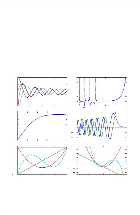
SciPy provides a plethora of special functions, including Bessel functions (and routines for finding their zeros, derivatives, and integrals), error functions, the gamma function, Legendre, Laguerre, and Hermite polynomials (and other polynomial functions), Mathieu functions, many statistical functions, and a number of other functions. Most are contained in the scipi.special library, and each has its own special arguments and syntax, depending on the vagaries of the particular function. We demonstrate a number of them in the code below that produces a plot of the different functions called. For more information, you should consult the SciPy web site on the scipy.special library.

Figure 9.1: Plots of special functions

Introduction to Python for Science, Release 0.9.23

1 import numpy as np

2import scipy as sp

3import matplotlib.pyplot as plt

4

5# create a figure window

6fig = plt.figure(1, figsize=(9,8))

7

8 # create arrays for a few Bessel functions and plot them

9x = np.linspace(0, 20, 256)

10j0 = sp.special.jn(0, x)

11j1 = sp.special.jn(1, x)

12y0 = sp.special.yn(0, x)

13y1 = sp.special.yn(1, x)

14ax1 = fig.add_subplot(321)

15ax1.plot(x,j0, x,j1, x,y0, x,y1)

16ax1.set_ylim(-1,1)

17ax1.text(0.5, 0.95,’Bessel’, ha=’center’, va=’top’,

18transform = ax1.transAxes)

19

20# gamma function

21x = np.linspace(-3.5, 6., 3601)

22g = sp.special.gamma(x)

23g = np.ma.masked_outside(g, -100, 400)

24ax2 = fig.add_subplot(322)

25ax2.plot(x,g)

26ax2.set_xlim(-3.5, 6)

27ax2.set_ylim(-20, 100)

28ax2.text(0.5, 0.95,’Gamma’, ha=’center’, va=’top’,

29transform = ax2.transAxes)

30

31# error function

32x = np.linspace(0, 2.5, 256)

33ef = sp.special.erf(x)

34ax3 = fig.add_subplot(323)

35ax3.plot(x,ef)

36ax3.set_ylim(0,1.1)

37ax3.text(0.5, 0.95,’Error’, ha=’center’, va=’top’,

38transform = ax3.transAxes)

39

40# Airy function

41x = np.linspace(-15, 4, 256)

42ai, aip, bi, bip = sp.special.airy(x)

43ax4 = fig.add_subplot(324)

44ax4.plot(x,ai, x,bi)

Introduction to Python for Science, Release 0.9.23

45ax4.axhline(color="grey", ls="--", zorder=-1)

46ax4.set_xlim(-15,4)

47ax4.set_ylim(-0.5,0.6)

48ax4.text(0.5, 0.95,’Airy’, ha=’center’, va=’top’,

49transform = ax4.transAxes)

50

51# Legendre polynomials

52x = np.linspace(-1, 1, 256)

53lp0 = np.polyval(sp.special.legendre(0),x)

54lp1 = np.polyval(sp.special.legendre(1),x)

55lp2 = np.polyval(sp.special.legendre(2),x)

56lp3 = np.polyval(sp.special.legendre(3),x)

57ax5 = fig.add_subplot(325)

58ax5.plot(x,lp0, x,lp1, x,lp2, x,lp3)

59ax5.axhline(color="grey", ls="--", zorder=-1)

60ax5.set_ylim(-1,1.1)

61ax5.text(0.5, 0.9,’Legendre’, ha=’center’, va=’top’,

62transform = ax5.transAxes)

63

64# Laguerre polynomials

65x = np.linspace(-5, 8, 256)

66lg0 = np.polyval(sp.special.laguerre(0),x)

67lg1 = np.polyval(sp.special.laguerre(1),x)

68lg2 = np.polyval(sp.special.laguerre(2),x)

69lg3 = np.polyval(sp.special.laguerre(3),x)

70ax6 = fig.add_subplot(326)

71ax6.plot(x,lg0, x,lg1, x,lg2, x,lg3)

72ax6.axhline(color="grey", ls="--", zorder=-1)

73ax6.axvline(color="grey", ls="--", zorder=-1)

74ax6.set_xlim(-5,8)

75ax6.set_ylim(-5,10)

76ax6.text(0.5, 0.9,’Laguerre’, ha=’center’, va=’top’,

77transform = ax6.transAxes)

78

79plt.show()

The arguments of the different functions depend, of course, on the nature of the particular function. For example, the first argument of the two types of Bessel functions called in lines 10-13 is the so-called order of the Bessel function, and the second argument is the independent variable. The Gamma and Error functions take one argument each and produce one output. The Airy function takes only one input argument, but returns four

outputs, which correspond the two Airy functions, normally designated Ai(x) and Bi(x), and their derivatives Ai0(x) and Bi0(x). The plot shows only Ai(x) and Bi(x).